Tree UGM Demo

In the last demo we considered chain-structured data, one of the simplest types of dependency where we can take advantage of the graphical structure to allow efficient decoding/inference/sampling. In this demo, we consider the case of tree-structured graphical models. In particular, we consider the case where the edges in the graph can be arbitrary, as long as the graph doesn't contain any loops. For models with this type of dependency structure, we can still perform efficient decoding/inference/sampling by applying generalizations of the methods designed for chain-structured models.

Water Turbidity Problem

In some cities, it occasionally happens that snow melting off of the mountain causes an increase in the turbidity of the drinking water at some locations. The turbidity level is used as a surrogate for testing whether the water is safe to drink. For this reason, we may want to build a probabilistic model of the water turbidity at different locations in the water system. We will do this with a UGM, where we use a tree-structured model to capture the dependencies between connected elements of the water system.

We will assume that turbidity is measured on a scale of 1 to 4, where 1 represents 'very safe', and 4 represents 'very unsafe'. We will assume that the water system can be represented by the following graph:

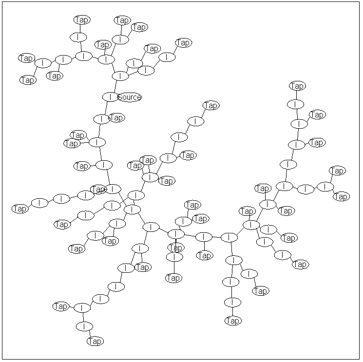
The node labeled 'Source' is the location where water enters the system. Similarly, the nodes labeled 'Tap' are locations where water exits the system, while nodes labeled 'I' are internal nodes. The graph structure above is a 'tree', meaning that there are no loops in the graph and the graph is connected (i.e., there exists a path of edges between all pairs of nodes).

We will assume that the node potentials for the source node are:

State Potential
1 0.9
2 0.09
3 0.009
4 0.001

That is, the water source will be 'very safe' 90% of the time, and 'very unsafe' 0.001% of the time. We will assign a unit value to all the other node potentials. For the edge potentials that describe the dependencies between adjacent nodes, we will use the following edge potential matrix:

From/to 1 2 3 4
1 0.9890 0.0099 0.0010 0.0001
2 0.1309 0.8618 0.0066 0.0007
3 0.0420 0.0841 0.8682 0.0057
4 0.0667 0.0333 0.1667 0.7333

In these edge potentials, the 'from' node represents the node that is closer to the source. The model assumes that the turdity level will generally be the same between adjacent nodes, with a small chance of it decreasing as we move away from the source, and an even smaller chance of it increasing as we move away from the source.

Representing the water system with UGM

As before, we first make the adjacency matrix and edgeStruct. Rather than typing out the large adjacency matrix, we will just load it from a .mat file: load('waterSystem.mat'); % Loads adj nNodes = length(adj); nStates = 4; edgeStruct = UGM_makeEdgeStruct(adj,nStates);
In the adjacency matrix, node 4 is the source node. We therefore make the nodpePot matrix using: source = 4; nodePot = ones(nNodes,nStates); nodePot(source,:) = [.9 .09 .009 .001];
Making the edgePot array is slightly more difficult, because we need to know which end of the edge is closer to the source. Further, if the 2nd node is closer to the source, we need to use the transpose of the edge potential matrix above. We do this is in a fairly simple (but not particularly efficient) way: transition = [ 0.9890 0.0099 0.0010 0.0001 0.1309 0.8618 0.0066 0.0007 0.0420 0.0841 0.8682 0.0057 0.0667 0.0333 0.1667 0.7333]; colored = zeros(nNodes,1); colored(source) = 1; done = 0; edgePot = zeros(nStates,nStates,edgeStruct.nEdges); while ~done done = 1; colored_old = colored; for e = 1:edgeStruct.nEdges if sum(colored_old(edgeStruct.edgeEnds(e,:))) == 1 % Determine direction of edge and color nodes if colored(edgeStruct.edgeEnds(e,1)) == 1 edgePot(:,:,e) = transition; else edgePot(:,:,e) = transition'; end colored(edgeStruct.edgeEnds(e,:)) = 1; done = 0; end end end

Decoding

In this model, we have 100 nodes that each can take 4 possible states, so we can't form a large table of possible states (with 4^100 elements) to do decoding as we did in the first demo. Further, our dependency structure is no longer a chain, so we can no longer use the Viterbi algorithm for decoding. Fortunately, the dynamic programming ideas used in the Viterbi algorithm can be extended to the case of a tree-structured dependency. This extension is often referred to as (max-product) belief propagation.

In the last demo, we mentioned that the forward-backward algorithms would give the same result if we reversed the order of the nodes. That is, instead of picking the last node as the 'end' and the first node as the 'start', we could have made the first node the 'end' and the last node the 'start', and we would get the same result. Towards extending this method to general trees, consider the following variation: we pick some node in the middle of the chain, and define this to be the 'end'. We then pick TWO 'start' nodes, the first node and the last node. We then run the forward pass of the algorithm starting from both 'start' nodes until both of these algorithms reach the 'end' node in the middle of the chain. We then combine the 'messages' coming from both directions, compute the optimal value of the 'end' node in the middle of the chain, and then 'backtrack' in both directions to get the optimal values for the rest of the chain.

It is straightforward to apply this idea to a general tree-structured graph:

We define some arbitrary node in the graph as the 'end' (or 'root') node
We define all nodes that have only one edge (excluding the 'root') as the 'start' nodes.
We run the 'max' version of the 'forward' algorithm starting from each 'start', moving towards the 'root' and merging results when we reach internal nodes.
Once the results from all the algorithms have been merged at the root, we backtrack through the tree to get the optimal decoding.

With UGM, we can run the max-product belief propagation algorithm on a tree-structured model using: optimalDecoding = UGM_Decode_Tree(nodePot,edgePot,edgeStruct)
In our model, the optimal decoding is that all nodes in the water system are 'very safe'.

Inference

We can make similar modifications to the forward-backward algorithm to get a 'sum-product' belief propagation algorithm that allows us to compute marginals and the normalizing constant. With UGM, we can run the sum-product belief propagation inference algorithm on a tree-structured model using: [nodeBel,edgeBel,logZ] = UGM_Infer_Tree(nodePot,edgePot,edgeStruct) nodeBel = 0.9103 0.0779 0.0110 0.0008 0.9110 0.0771 0.0111 0.0008 0.9129 0.0750 0.0114 0.0008 0.9000 0.0900 0.0090 0.0010 0.9073 0.0814 0.0104 0.0008 0.9129 0.0750 0.0114 0.0008 0.9116 0.0764 0.0112 0.0008 0.9085 0.0800 0.0106 0.0008 0.9043 0.0850 0.0099 0.0009 0.9085 0.0800 0.0106 0.0008 0.9129 0.0750 0.0114 0.0008 0.9121 0.0759 0.0112 0.0008 0.9141 0.0736 0.0115 0.0008 0.9110 0.0771 0.0111 0.0008 0.9085 0.0800 0.0106 0.0008 0.9059 0.0830 0.0102 0.0009 0.9073 0.0814 0.0104 0.0008 0.9103 0.0779 0.0110 0.0008 0.9125 0.0754 0.0113 0.0008 0.9116 0.0764 0.0112 0.0008 0.9138 0.0739 0.0115 0.0008 0.9125 0.0754 0.0113 0.0008 0.9085 0.0800 0.0106 0.0008 0.9103 0.0779 0.0110 0.0008 0.9095 0.0789 0.0108 0.0008 0.9132 0.0746 0.0114 0.0008 0.9129 0.0750 0.0114 0.0008 0.9129 0.0750 0.0114 0.0008 0.9116 0.0764 0.0112 0.0008 0.9129 0.0750 0.0114 0.0008 0.9116 0.0764 0.0112 0.0008 0.9110 0.0771 0.0111 0.0008 0.9116 0.0764 0.0112 0.0008 0.9121 0.0759 0.0112 0.0008 0.9140 0.0737 0.0115 0.0008 0.9132 0.0746 0.0114 0.0008 0.9121 0.0759 0.0112 0.0008 0.9073 0.0814 0.0104 0.0008 0.9116 0.0764 0.0112 0.0008 0.9116 0.0764 0.0112 0.0008 0.9134 0.0743 0.0114 0.0008 0.9073 0.0814 0.0104 0.0008 0.9134 0.0743 0.0114 0.0008 0.9095 0.0789 0.0108 0.0008 0.9138 0.0739 0.0115 0.0008 0.9125 0.0754 0.0113 0.0008 0.9132 0.0746 0.0114 0.0008 0.9116 0.0764 0.0112 0.0008 0.9095 0.0789 0.0108 0.0008 0.9134 0.0743 0.0114 0.0008 0.9073 0.0814 0.0104 0.0008 0.9059 0.0830 0.0102 0.0009 0.9138 0.0739 0.0115 0.0008 0.9116 0.0764 0.0112 0.0008 0.9132 0.0746 0.0114 0.0008 0.9140 0.0737 0.0115 0.0008 0.9059 0.0830 0.0102 0.0009 0.9103 0.0779 0.0110 0.0008 0.9132 0.0746 0.0114 0.0008 0.9132 0.0746 0.0114 0.0008 0.9110 0.0771 0.0111 0.0008 0.9095 0.0789 0.0108 0.0008 0.9132 0.0746 0.0114 0.0008 0.9073 0.0814 0.0104 0.0008 0.9137 0.0741 0.0115 0.0008 0.9116 0.0764 0.0112 0.0008 0.9059 0.0830 0.0102 0.0009 0.9134 0.0743 0.0114 0.0008 0.9138 0.0739 0.0115 0.0008 0.9023 0.0873 0.0095 0.0009 0.9116 0.0764 0.0112 0.0008 0.9103 0.0779 0.0110 0.0008 0.9125 0.0754 0.0113 0.0008 0.9121 0.0759 0.0112 0.0008 0.9085 0.0800 0.0106 0.0008 0.9073 0.0814 0.0104 0.0008 0.9116 0.0764 0.0112 0.0008 0.9121 0.0759 0.0112 0.0008 0.9095 0.0789 0.0108 0.0008 0.9134 0.0743 0.0114 0.0008 0.9137 0.0741 0.0115 0.0008 0.9116 0.0764 0.0112 0.0008 0.9110 0.0771 0.0111 0.0008 0.9129 0.0750 0.0114 0.0008 0.9121 0.0759 0.0112 0.0008 0.9059 0.0830 0.0102 0.0009 0.9085 0.0800 0.0106 0.0008 0.9095 0.0789 0.0108 0.0008 0.9132 0.0746 0.0114 0.0008 0.9121 0.0759 0.0112 0.0008 0.9085 0.0800 0.0106 0.0008 0.9129 0.0750 0.0114 0.0008 0.9110 0.0771 0.0111 0.0008 0.9103 0.0779 0.0110 0.0008 0.9110 0.0771 0.0111 0.0008 0.9073 0.0814 0.0104 0.0008 0.9043 0.0850 0.0099 0.0009 0.9132 0.0746 0.0114 0.0008 0.9121 0.0759 0.0112 0.0008 0.9121 0.0759 0.0112 0.0008
We see in row 4 that the source node's marginals match its node potentials. We also see that the probability of the water being 'very safe' is higher than the source's maginals for all other nodes, while the probability of the other levels is decreased.

In this specific model, the node potentials of the source node can be interpreted as a marginal probability and the values of the edge potentials can be interpreted as transition probabilities. Further, it is possible to use simpler forward inference and sampling methods, similar to the Chapman-Kolmogorov equations for Markov chains (in this case, we apply the analogous equations to an appropriately defined branching process, where we start at the source, branch at internal nodes, and terminate at tap nodes). This probabilistic interpretation will not hold for general tree-structured UGMs. However, the methods implemented in UGM handle the case of general tree-structured UGMs, and can therefore handle the extensions to non-unit potentials (beyond the source node), or edge potentials that aren't normalized probabilities as we move away from the source.

Sampling

Sampling from a tree-structured UGM is again a straightforward extension of the forwards-filter backwards-sample algorithm for chain-structured UGMs. With UGM, we can generate 100 samples from a tree-structured model using: edgeStruct.maxIter = 100; samples = UGM_Sample_Tree(nodePot,edgePot,edgeStruct);
Here is a visualization of 100 samples:

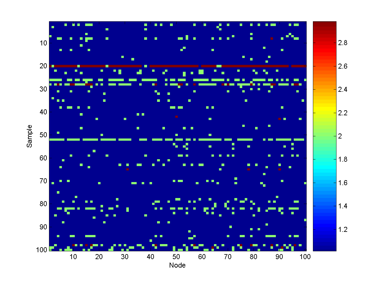
From these samples, we see that turbidity can spread widely throughout the water system, depending on how far the source is from the 'very safe' state.

Notes

Since chains are a special case of trees, for the last two demos we could have used the tree decoding/inference/sampling methods discussed in this demo. Further, the tree decoding/inference/sampling methods implemented in UGM can handle the case of 'forests'. A forest-structured graph is a graph that has no loops. This generalizes tree-structured graphs, because the forests do not need to be connected. Said another way, a forest is a union of non-overlapping tree-structured graphs.

In the samples generated above, the state '4' was never encountered. Although we would eventually generate samples where state 4 was encountered, knowing how the model behaves in this scenario is clearly important and we may not want to wait for these unlikely scenarios to occur. In the next demo, we examine performing conditional decoding/inference/sampling, where we perform these operations under the assumption that the values of one or more nodes are known (ie. what happens to the other nodes when the source node is in state 4).

PREVIOUS DEMO NEXT DEMO

Mark Schmidt > Software > UGM > Tree Demo

From/to	1	2	3	4
1	0.9890	0.0099	0.0010	0.0001
2	0.1309	0.8618	0.0066	0.0007
3	0.0420	0.0841	0.8682	0.0057
4	0.0667	0.0333	0.1667	0.7333