Chain UGM Demo
The naive
methods for decoding/inference/sampling discussed in the previous demo
require exponential time in both the number of nodes and the number of states,
so they
are completely impractical if the number of nodes or the number of states is non-trivial.
In this demo, we consider the case where the graph structure is a chain. By
taking advantage of the conditional independence properties induced by the chain
structure, it is possible to derive polynomial-time methods for
decoding/inference/sampling. These methods can be applied even when the chain
is very long, and when each node in the chain can take many values.
Computer Science Graduate Careers
In this demo, we will build a simple Markov chain model of what people do after they graduate with a computer science degree. In this model, we will assume that every new computer science grad initially starts out in
one of three states:
| State | Probability | Description
|
| Industry | 0.60 | They work for a company or own their
own company.
|
| Grad School | 0.30 | They are trying to get a Masters or
PhD degree.
|
| Video Games | 0.10 | They mostly play video games.
|
After each year, the grad can either stay in the same state, or transition to a different state. We will build a model for the
first sixty years after graduation. Besides the three possible initial
states above, we will also consider four states that you could transition into:
| State | Description
|
| Industry (with PhD) | They work for a company or own their
own company, and have a PhD.
|
| Academia | They work as a post-doctoral researcher or professor.
|
| Video Games (with PhD) | They mostly play video games, but have a PhD.
|
| Deceased | They no longer work in computer science.
|
Note that we haven't yet stated the probability of transitioning into each of these
states, since we will make these probabilities depend on
what state you were in for the last year. For example, you can only transition
to the states requiring a PhD if your last state was 'Grad School' or another
state where you have a PhD. Another example is the 'Deceased' state, since
once you are in this state, you remain in it. Because of this, the 'Deceased' state is known as an 'absorbing
state'.
In this model, we make a crucial assumption about transitioning into new
states. We assume that the probability of transitioning into your new state
depends only on your previous state. This implies a conditional independence between the current year and all previous years, given the value of the last year.
We will assume the following state
transition matrix:
| From\to | Video Games | Industry | Grad School | Video Games (with PhD) | Industry (with
PhD) | Academia | Deceased
|
| Video Games | 0.08 | 0.90 | 0.01 | 0 | 0 | 0 | 0.01
|
| Industry | 0.03 | 0.95 | 0.01 | 0 | 0 | 0 | 0.01
|
| Grad School | 0.06 | 0.06 | 0.75 | 0.05 | 0.05 | 0.02 | 0.01
|
| Video Games (with PhD) | 0 | 0 | 0 | 0.30 | 0.60 | 0.09 | 0.01
|
| Industry (with PhD) | 0 | 0 | 0 | 0.02 | 0.95 | 0.02 | 0.01
|
| Academia | 0 | 0 | 0 | 0.01 | 0.01 | 0.97 | 0.01
|
| Deceased | 0 | 0 | 0 | 0 | 0 | 0 | 1
|
The row gives the state we are transitioning from, and the column gives the state
we are transitioning to. For example, our model assumes that the probability
of transitioning from 'Industry' to 'Video Games' is 0.03, the
probability of transitioning from 'Grad School' to 'Academia' is 0.02, the
probability of transitioning from 'Academia' to 'Academia' is 0.97, etc.
Representing a Markov chain with UGM
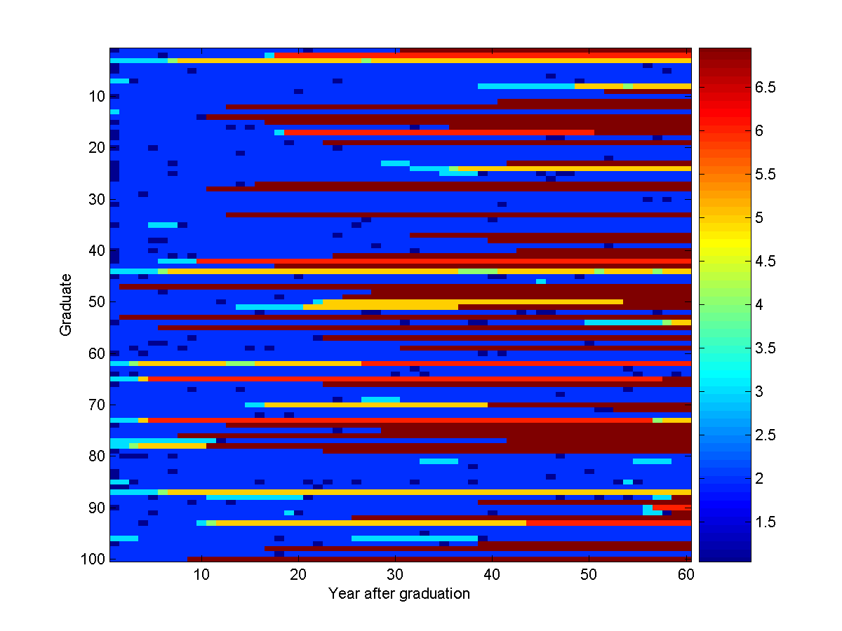
The model described above is known as a Markov chain. Usually, we write the
joint likelihood for a sequence of variables in a Markov chain as:
p(x1) comes from the initial distribution, while
p(xi|xi-1) comes from the transition matrix.
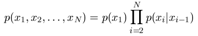
We now consider representing this Markov chain model with an equivalent UGM.
We will
make each node
represent a year, and each node can take one of the 7 states described above.
We place edges between nodes representing adjacent years (ie. year '3' is
connected to years '2' and '4').
Thus, to make the edgeStruct that describes the time dependency between the
nodes, we use:
nNodes = 60;
nStates = 7;
adj = zeros(nNodes);
for i = 1:nNodes-1
   adj(i,i+1) = 1;
end
adj = adj+adj';
edgeStruct = UGM_makeEdgeStruct(adj,nStates);
If Graphviz is installed, we can use the 'drawGraph'
function to visualize the adjacency matrix:
drawGraph(adj);
We now make the nodePot matrix. The initial distribution will be reflected in
the node potentials for the first state:
initial = [.3 .6 .1 0 0 0 0];
nodePot = zeros(nNodes,nStates);
nodePot(1,:) = initial;
nodePot(2:end,:) = 1;
We set the node potentials for the remaining states to the constant value '1'. We did this to remove the influence of the remaining node potentials on the distribution.
For the edgePot array, we copy our transition matrix above, and replicate it
for each transition:
transitions = [.08 .9 .01 0 0 0 .01
    .03 .95 .01 0 0 0 .01
    .06 .06 .75 .05 .05 .02 .01
    0 0 0 .3 .6 .09 .01
    0 0 0 .02 .95 .02 .01
    0 0 0 .01 .01 .97 .01
    0 0 0 0 0 0 1];
edgePot = repmat(transitions,[1 1 edgeStruct.nEdges]);
In general we can not interpret the potentials in a UGM as representing probabilities, but in this case we have carefully constructed the UGM so that the node potentials are equal to the initial probabilities p(xi) and the edge potentials are equal to the transition probabilities p(xi|xi-1) in a Markov chain. If we
changed the node potentials to be non-identical after the first state, or we changed
the edge potentials so that they don't sum to 1 across rows, then the model
would still be equivalent to a Markov chain, but the node/edge potentials would
no longer be equal to these probabilities in the model.
Decoding
In this model, we have 60 nodes, and each of these can take 7 possible states. This means that there are total of 7^60 possible configurations of the states. Thus, unlike the previous demo, it is completely infeasible to write out all of the
possible states. It might also appear unrealistic to even do things
like decoding, since this involves finding the maximum among the 7^60 possible states.
Fortunately, the Markov property means that most of the calculations we would
do in computing this maximum are redundant. That is, some parts of the
calculation are repeated many times. By taking advantage of this
with standard techniques from dynamic programming, we can reduce the
search over all 7^60 states down to a simple polynomial-time algorithm.
In particular, the Viterbi algorithm implements a dynamic programming strategy that only requires O(nNodes*nStates^2) time.
Roughly, it consists of two phases:
- Forward Phase: We go through the states from beginning to end. When we get to node 'n', we compute the maximum potential that we achieve by assigning node 'n' to each of its possible states, based only on the first 'n' node potentials and the edge potentials for edges between these nodes. For the first node this is trivial, we just take the first row of the nodePot matrix and normalize it. For subsequent nodes, we consider all combinations of node 'n' with the maximum values achieved by node 'n-1' to compute the best value of node 'n' in time O(nStates^2).
- Backward Phase: Once we get to the end, we can easily tell what the best value of the last
state is. We then 'backtrack' through the sequence from end to beginning,
reading off the states that lead to the best sequence.
With UGM, we can run Viterbi decoding on a chain-structured model using:
optimalDecoding = UGM_Decode_Chain(nodePot,edgePot,edgeStruct)
Unfortunately, the optimal decoding in this particular model is not very interesting: it is a string of
2's. That is, the most likely sequence of states is that a CS grad will start
in 'Industry', and stay in it for 60 years. However, even though
this is the most likely sequence, it doesn't look anything like samples that
actually occur in the model. This is because, in the big 7^60 element
probability table, the most probable value still isn't all that probable. It
is also interesting to note that the most likely sequence would change if we looked at a longer timeframe.
Inference
Because of the way we constructed the model, the marginals in the first state are trivially [.3 .6 .1 0
0 0 0]. A simple way to compute the marginals for future states in a Markov chain is with
the Chapman-Kolmogorv
equations, which for problems with a finite number of states corresponds to matrix multiplication of the initial probabilities with the transition matrix. For example, to compute the marginals in the second, third,
and fourth states, we would use:
initial*transitions

ans =

    0.0480    0.8460    0.0840    0.0050    0.0050    0.0020    0.0100

initial*transitions^2

ans =

    0.0343    0.8519    0.0719    0.0058    0.0120    0.0042    0.0199

initial*transitions^3

ans =

    0.0326    0.8445    0.0628    0.0056    0.0185    0.0062    0.0297
However, this will not work for all chain-structure UGMs. For example, we
might have non-uniform node potentials after the first state.
Such a model
might encode things like the potential of being 'Deceased' increases over
time while the potential of being in 'Grad School' decreases over time.
Another widely-used chain-structured UGM where the
Chapman-Kolomogorv equations don't apply is hidden Markov
models. We could consider converting
these UGMs into Markov chains and then using the Chapman-Kolomogorv equations for
inference, but this actually requires inference to get the probabilities.
Fortunately, we can efficiently and directly compute marginals in general chain-structured UGMs using the forwards-backwards algorithm. As with Viterbi
decoding (and as its name would suggest), the forwards-backwards algorithm has
two phases: (i) a forwards phase where we go through the nodes from start to
end, and (ii) a backwards phase where we use information from the end of the
sequence to work our way back to the beginning.
The forward phase is nearly identical to Viterbi decoding. We start with the
first node, and compute its marginal probability for each state, ignoring all
node/edge potentials that involve other states. We then move on to the second node,
and compute its marginal probability for each state (ignoring all node/edge
potentials that involve nodes other than the first two), using the 'message' of
marginal probabilities computed for the first state. Thus, the forward phase
of the forward-backwards algorithm is similar to the forwards phase of Viterbi
decoding, except we are computing (normalized) sums instead of maximums. Here,
the computational gain comes from aggregating the sums from multiple paths that lead
to the same state.
Once the forward phase is complete, we obtain the actual marginal probabilities for
the last state (since this state takes into account all the node/edge
potentials for all 7^60 paths). We can
also get the normalizing constant Z, which will be the product of the constants
we use to normalize each of the marginals computed during the forward phase
(alternately, we could leave the individual marginals unnormalized, and in this
case Z would be the sum of the unnormalized marginals of the last state).
We are typically interested in computing the marginals of states other than the
last state, and the backward phase is what allows us to do this. The backward
phase is very similar to the forward phase, except that we go through the
sequence backwards and send a slightly different type of message. In fact,
there are versions of the forwards-backwards algorithm where the forward and
backward phases are identical (and can be run in parallel). Once the backward
phase is complete, we can compute all the node marginals by normalizing the
product of the forward and backward messages.
With UGM, we can run the forward-backwards inference algorithm on a chain-structured model using:
[nodeBel,edgeBel,logZ] = UGM_Infer_Chain(nodePot,edgePot,edgeStruct)
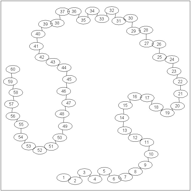
Let's take a look at the computed node marginals:
nodeBel =

    0.3000    0.6000    0.1000         0         0         0         0
    0.0480    0.8460    0.0840    0.0050    0.0050    0.0020    0.0100
    0.0343    0.8519    0.0719    0.0058    0.0120    0.0042    0.0199
    0.0326    0.8445    0.0628    0.0056    0.0185    0.0062    0.0297
    0.0317    0.8354    0.0559    0.0053    0.0242    0.0082    0.0394
    0.0310    0.8255    0.0506    0.0049    0.0290    0.0100    0.0490
    0.0303    0.8151    0.0465    0.0047    0.0331    0.0118    0.0585
    0.0297    0.8044    0.0433    0.0045    0.0367    0.0134    0.0679
    0.0291    0.7935    0.0408    0.0044    0.0399    0.0150    0.0773
    0.0286    0.7825    0.0389    0.0043    0.0427    0.0166    0.0865
    0.0281    0.7714    0.0373    0.0043    0.0453    0.0181    0.0956
    0.0276    0.7603    0.0359    0.0042    0.0476    0.0196    0.1047
    0.0272    0.7493    0.0348    0.0042    0.0498    0.0211    0.1136
    0.0267    0.7384    0.0339    0.0042    0.0518    0.0225    0.1225
    0.0263    0.7276    0.0331    0.0042    0.0536    0.0239    0.1313
    0.0259    0.7169    0.0323    0.0042    0.0554    0.0253    0.1399
    0.0255    0.7063    0.0317    0.0042    0.0570    0.0267    0.1485
    0.0251    0.6959    0.0311    0.0043    0.0585    0.0280    0.1571
    0.0248    0.6856    0.0305    0.0043    0.0600    0.0294    0.1655
    0.0244    0.6754    0.0300    0.0043    0.0614    0.0307    0.1738
    0.0240    0.6654    0.0295    0.0043    0.0627    0.0320    0.1821
    0.0237    0.6555    0.0290    0.0043    0.0640    0.0333    0.1903
    0.0233    0.6457    0.0286    0.0044    0.0652    0.0345    0.1984
    0.0229    0.6361    0.0281    0.0044    0.0663    0.0357    0.2064
    0.0226    0.6267    0.0277    0.0044    0.0674    0.0370    0.2143
    0.0223    0.6173    0.0272    0.0044    0.0684    0.0381    0.2222
    0.0219    0.6081    0.0268    0.0044    0.0694    0.0393    0.2300
    0.0216    0.5991    0.0264    0.0045    0.0703    0.0405    0.2377
    0.0213    0.5902    0.0260    0.0045    0.0712    0.0416    0.2453
    0.0210    0.5814    0.0256    0.0045    0.0720    0.0427    0.2528
    0.0207    0.5727    0.0252    0.0045    0.0728    0.0438    0.2603
    0.0203    0.5642    0.0249    0.0045    0.0736    0.0448    0.2677
    0.0200    0.5558    0.0245    0.0045    0.0743    0.0458    0.2750
    0.0197    0.5475    0.0241    0.0045    0.0750    0.0468    0.2823
    0.0195    0.5394    0.0238    0.0045    0.0756    0.0478    0.2894
    0.0192    0.5313    0.0234    0.0045    0.0762    0.0488    0.2966
    0.0189    0.5234    0.0231    0.0045    0.0768    0.0497    0.3036
    0.0186    0.5156    0.0227    0.0045    0.0773    0.0506    0.3106
    0.0183    0.5079    0.0224    0.0046    0.0778    0.0515    0.3174
    0.0180    0.5004    0.0221    0.0046    0.0783    0.0524    0.3243
    0.0178    0.4929    0.0217    0.0046    0.0788    0.0532    0.3310
    0.0175    0.4856    0.0214    0.0046    0.0792    0.0541    0.3377
    0.0173    0.4783    0.0211    0.0046    0.0796    0.0549    0.3443
    0.0170    0.4712    0.0208    0.0046    0.0799    0.0556    0.3509
    0.0167    0.4642    0.0205    0.0046    0.0803    0.0564    0.3574
    0.0165    0.4573    0.0202    0.0046    0.0806    0.0571    0.3638
    0.0162    0.4505    0.0199    0.0046    0.0809    0.0578    0.3702
    0.0160    0.4438    0.0196    0.0046    0.0811    0.0585    0.3765
    0.0158    0.4371    0.0193    0.0046    0.0814    0.0592    0.3827
    0.0155    0.4306    0.0190    0.0045    0.0816    0.0598    0.3889
    0.0153    0.4242    0.0187    0.0045    0.0818    0.0605    0.3950
    0.0151    0.4179    0.0184    0.0045    0.0820    0.0611    0.4010
    0.0148    0.4117    0.0181    0.0045    0.0821    0.0617    0.4070
    0.0146    0.4055    0.0179    0.0045    0.0822    0.0622    0.4130
    0.0144    0.3995    0.0176    0.0045    0.0824    0.0628    0.4188
    0.0142    0.3936    0.0173    0.0045    0.0825    0.0633    0.4246
    0.0140    0.3877    0.0171    0.0045    0.0826    0.0638    0.4304
    0.0138    0.3819    0.0168    0.0045    0.0826    0.0643    0.4361
    0.0136    0.3762    0.0166    0.0045    0.0827    0.0647    0.4417
    0.0134    0.3706    0.0163    0.0045    0.0827    0.0652    0.4473
Or more visually:
Notice that the first four states match the results we got with the
Chapman-Kolmogorov equations. In general, the node marginals give us more information about the process than the optimal
decoding. For example, while the optimal decoding told us that the most likely
scenario was for someone to stay industry for 60 years, the node marginals tell
us that the probability of being in industry after 60 is only .3706, while the
probability of being deceased is 0.4473. Further, the probability of someone being
deceased in our model is higher than the probability of staying in industry for
the last 7 states. We can also use the
node marginals to answer questions such as "what is the probability of being
in academia after 10 years or 20 years?" (0.0166, 0.0294).
If we kept going further into the future, the node marginals would eventually
converge to the stationary distribution, corresponding to the left eigenvector
of the transition matrix
with the largest eigenvalue. For our Markov chain, this eigenvector is [0 0 0
0 0 0 1], meaning that everyone eventually ends up in the 'absorbing state'.
Sampling
Sampling in a Markov chain is simple: we first generate a state from the initial
distribution, then we generate the next state using the appropriate row from
the transition matrix, and then we repeat this until we reach the end of the
sequence. This is a fairly intuitive process, we basically just simulate
someone's life according to the probabilities from the initial distribution and our transition matrix.
However, as with the
Chapman-Kolmogorv equations, we can't apply this procedure to general
chain-structure UGMs (unless we convert the UGM to an equivalent Markov chain first...).
To directly sample from a general chain-structured UGM, we can use the foward-filter
backward-sample algorithm. This algorithm is not as well known as the Viterbi
and forwards-backwards algorithm, it does not even have a Wikipedia page yet. It
is described in these papers:
- C.K. Carter and R. Kohn. On Gibbs sampling for state space models. Biometrika, 1994.
- S. Früwirth-Schnatter. Data augmentation and dynamic linear models. Journal of Times Series Analysis, 1994.
- S. Chib. Calculating posterior distributions and modal estimates in
Markov mixture models. Journal of Econometrics, 1996.
The forward phase of this algorithm is identical to the forward phase of the
forward-backward algorithm. In the backward phase, we first generate a state
from the last node's marginal distribution. Then, we move to the second last
node, and generate its state using the forward message and conditioning on the
sample of the last state. We continue this process backwards through the chain
until we have finally generated a sample for the first node.
This computational procedure is less intuitive than the simple forward-sampling
procedure for Markov chains. For example, consider the case where our sample of the
last state from its node marginal gives us 'Video Games' (the node marginals
tell us that this happens with probability 0.0134). Given this state, we
now go backwards in time and sample a 59th state according to its
probability of occuring starting from the beginning, combined with our
knowledge that it must lead to the state 'Video Games'. The magical part of this algorithm is that when we have gone back in time far enough
to reach the very first state, the first state will still be drawn from our [.3
.6 .1] initial distribution. The UGM, being undirected, doesn't care
that we are simulating someone's life backwards. In fact, if we reversed the sequence,
then the backward phase would exactly implement the simple forward sampler.
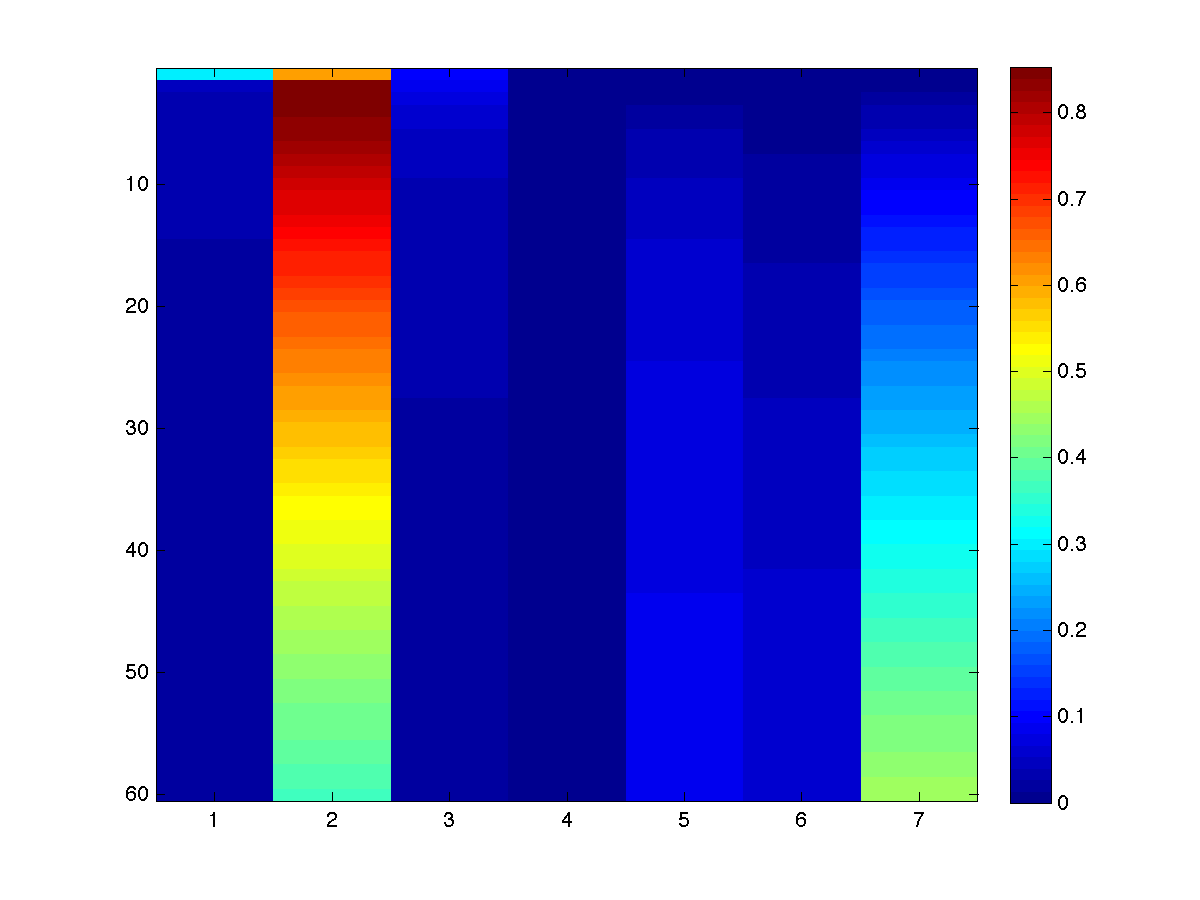
With UGM, we can run the forward-filter backward-sample algorithm to generate
100 samples using:
edgeStruct.maxIter = 100;
samples = UGM_Sample_Chain(nodePot,edgePot,edgeStruct);
imagesc(samples');
xlabel('Year after graduation');
ylabel('Graduate');
colorbar
So, under our model, here is what 100 computer science graduates do in their first 60 years after graduating:
Recall the numbers we assigned to the states: (1) Video Games, (2) Industry, (3) Grad School,
(4) Video Games (with PhD), (5) Industry (with PhD), (6) Academia, (7) Deceased.
Note that the most likely sequence (staying in Industry for 60 years) didn't
occur in any of these samples.
Notes
In our Markov chain, we assumed that the transition matrix is the same for
every edge (however, unlike the first demo, we did not assume it was symmetric).
This is known as a homogeneous Markov chain. If we wanted a more
realistic model, we might consider having a set of transition probabilities
that change over time. For example, we might want to decrease the probability of
transitioning into the 'Grad School' state as people age.
We close by noting that in the first demo, a chain
structure was also used. Therefore, using the chain
decoding/inference/sampling methods will give the same results as the brute
force methods used in that demo.
PREVIOUS DEMO NEXT DEMO
Mark Schmidt > Software > UGM > Chain Demo