Condition UGM Demo
In the previous three demos, we considered the unconditional
decoding/inference/sampling tasks. That is, we assumed that we don't know
the values of any of the random variables in the model. However, in many
cases, we will want to consider what happens when we know the value of one or more of the random variables. That
is, we have 'observations' and we want to do conditional
decoding/inference/sampling.
For example, we might want to answer queries about the three previous demos like:
- Demo 1: If Mark and Cathy get the question wrong, what is the probability that
Heather still gets the question right?
- Demo 2: What is the most likely path of a CS graduate's career, given that
he is in academia 10 years after graduating? And what do samples of his
career look like?
- Demo 3: What happens to the rest of the water system if the source node is in
state 4? If we use a model with multiple sources and observe that one of the
nodes is in state 4, which source is more likely to also be in an unsafe state?
Conditioning
UGMs are closed under conditioning. This means that if we condition on the values of
some of the variables, the resulting distribution will still be a UGM.
For example, consider the
4-node UGM with a chain-structured dependency 1-2-3-4, and
the case where we want to
condition on nodes 2 and 3.
We obtain:
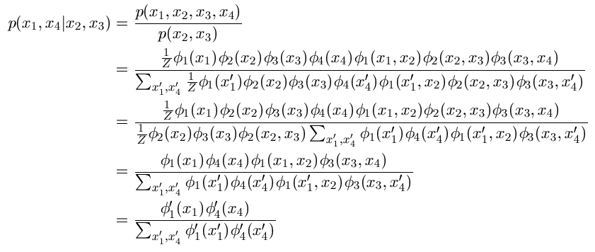
In the first line, we use the definition of conditional probability, while the
second line uses the definition of the UGM. In the third line, we take terms
not depending on the summation index outside of the summation in the denominator,
and we cancel out these terms in the fourth line. Finally, in the fifth line,
we define a new potential phi'1 that is equal to
phi1(x1) times
phi1(x1,x2), while phi'4 is defined
analogously to absorb the potential coming from the 3-4 edge.
Thus, the conditional probability of {1,4} given {2,3} is a
UGM defined on {1,4}.
In general, we can convert an unconditional UGM into a UGM
representing conditional probabilities with the following simple procedure:
- We remove the nodes (and corresponding node potentials) for observed nodes from the model
- We remove the edges (and corresponding edge potentials) between observed nodes from the model.
- For each edge between an observed node and a regular node, we
element-wise multiply the node potential of the regular node by the relevant row or column of the edge
potential, and then remove the edge (and corresponding edge potential) from the model.
- We now have no terms left depending on the observed nodes, so the normalizing constant is the sum over regular nodes only.
Note that the conditional UGM will be defined on the subgraph of the original graph corresponding to the unobserved nodes.
This is an important property to keep in mind, since the subgraph may have a simpler structure that the original graph.
In the example above, there are no edges in the conditional UGM, which makes it trivial to do decoding/inference/sampling.
Forming the Conditional UGM
The function UGM_makeClampedPotentials implements the above procedure.
It requires 4 inputs: the nodePot matrix, the edgePot array, the edgeStruct,
and the clamped vector. The clamped variable is a nNodes-by-1 vector where element i is set to the observed state if a node is observed, and is set to 0 for unobserved variables.
For example, to form the conditional UGM after conditioning on
the observations that node 2 is set to state 1 and node 3 is set to state 2, we
type:
clamped = zeros(nNodes,1);
clamped(2) = 1;
clamped(3) = 2;
[condNodePot,condEdgePot,condEdgeStruct,edgeMap] = UGM_makeClampedPotentials(nodePot,edgePot, edgeStruct, clamped);
This function returns the UGM representation of the 'conditional' UGM:
condNodePot gives the conditional node potentials, condEdgePot gives the
conditional edge potentials, and condEdgeStruct gives the edgeStruct for the
conditional adjacency matrix. With these modified potentials and edgeStruct,
we can now apply decoding/inference/sampling methods to the conditional UGM to
answer conditional queries about the original UGM.
Since some nodes and edges will be missing from the conditional UGM, you need
to be careful about node and edge numbers. In the example above, condNodePot
will have 2 rows deleted, since nodes 2 and 3 are removed from the original model.
To track edges between the original and
conditional model, the
edgeMap variable is a vector where each row gives the edge number in the
original model of those edges present in the conditional model.
Conditional Decoding/Inference/Sampling
In many cases, we may be interested in various aspects of the conditional UGM,
and in these case we need to worry about the above indexing issue.
However, if we are simply interested in doing conditional
decoding/inference/sampling and expressing the results in terms of the original
variables, UGM provides three functions that implement the relevant
conditioning and indexing/de-indexing operations. These three functions use a similar format to the other decoding/inference/sampling functions we have
examined, but take two additional input arguments:
- They require the
clamped vector described above that gives the values of the observed nodes.
- They require an anonymous function that will do the
decoding/inference/sampling on the conditional UGM.
UGM's conditional decoding/inference/sampling methods automatically build the conditional UGM, use the anonymous function as a sub-routine to do decoding/inference/sampling in the conditional UGM, and then expresses the results in terms of the original variables. Thus, we can use any decoding/inference/sampling that works with the conditional UGM structure.
We now demonstrate the use of these functions with a few examples.
We want to know what the probability of Heather getting the question right is,
given that Mark and Cathy got the question wrong. First, we make the
cheating students UGM:
nNodes = 4;
adj = zeros(nNodes);
adj(1,2) = 1;
adj(2,3) = 1;
adj(3,4) = 1;
adj = adj + adj';
nStates = 2;
edgeStruct = UGM_makeEdgeStruct(adj,nStates);
nodePot = [1 3
    9 1
    1 3
    9 1];
edgePot = zeros(nStates,nStates,edgeStruct.nEdges);
edgePot(:,:,1) = [2 1 ; 1 2];
edgePot(:,:,2) = [2 1 ; 1 2];
edgePot(:,:,3) = [2 1 ; 1 2];
We now make the clamped vector, where the answers that Cathy (1) and Mark (3)
give are clamped to the 'wrong' (2) state:
clamped = zeros(nNodes,1);
clamped(1) = 2;
clamped(3) = 2;
We now do conditional inference, where we use UGM_Infer_Exact as
the anonymous inference function:
[nodeBel,edgeBel,logZ] = UGM_Infer_Conditional(nodePot,edgePot,edgeStruct,clamped,@UGM_Infer_Exact);

nodeBel =

         0    1.0000
    0.6923    0.3077
         0    1.0000
    0.8182    0.1818
Obviously, since we observe that Cathy and Mark get the question wrong, their
probability of getting it wrong is 1 and of getting it right is 0. From these
node marginals, we see that the probability of Heather getting the question
right given that Mark and Cathy got the question wrong is only ~0.69 (compard
to 0.90 when Heather didn't see their answers, and ~0.84 if we don't know the
values of Cathy and Mark's answers). We could
also compute the probability that Heather gets the question right if Mark and
Cathy guessed the right answer:
clamped(1) = 1;
clamped(3) = 1;
[nodeBel,edgeBel,logZ] = UGM_Infer_Conditional(nodePot,edgePot,edgeStruct,clamped,@UGM_Infer_Exact);

nodeBel =

    1.0000         0
    0.9730    0.0270
    1.0000         0
    0.9474    0.0526
In this case, the probability of Heather getting the question right is
increased to ~0.97. We might also want to know what the probability of Heather getting
the question right is if Allison also gets it right (in addition to Cathy and
Mark). However, Heather is independent of Allison in the conditional UGM
(since there is no path between them in the conditional graph), so it would remain
~0.97.
If someone is in academia 10 years after graduating, we want to know what their
most likely path through the 60 years is, and what samples of their future
will look like. To do this, we first make the graduate careers UGM:
nNodes = 60;
nStates = 7;
adj = zeros(nNodes);
for i = 1:nNodes-1
   adj(i,i+1) = 1;
end
adj = adj+adj';
edgeStruct = UGM_makeEdgeStruct(adj,nStates);
initial = [.3 .6 .1 0 0 0 0];
nodePot = zeros(nNodes,nStates);
nodePot(1,:) = initial;
nodePot(2:end,:) = 1;
transitions = [.08 .9 .01 0 0 0 .01
    .03 .95 .01 0 0 0 .01
    .06 .06 .75 .05 .05 .02 .01
    0 0 0 .3 .6 .09 .01
    0 0 0 .02 .95 .02 .01
    0 0 0 .01 .01 .97 .01
    0 0 0 0 0 0 1];
edgePot = repmat(transitions,[1 1 edgeStruct.nEdges]);
We now make the clamped vector, where we clamp the value of the 10th state to
'Academia' (6):
clamped = zeros(nNodes,1);
clamped(10) = 6;
Now, to get the most likely sequence that includes this state, we want to do
conditional decoding. However, we need to be careful about what function we
use to do this decoding. This is because we remove the 10th node from the
UGM to make the conditional UGM, so the conditional UGM is no longer a chain.
Therefore, we can't use UGM_Decode_Chain as our anonymous decoding function,
since the conditional UGM will be comprised of two independent chains. Because
these independent chains form a 'forest' graph structure, we will instead use
the UGM_Decode_Tree function:
optimalDecoding = UGM_Decode_Conditional(nodePot,edgePot,edgeStruct,clamped,@UGM_Decode_Tree);

optimalDecoding =

     3
     6
     6
     6
     6
     6
     6
     6
     6
     6
     6
     6
     6
     6
     6
     6
     6
     6
     6
     6
     6
     6
     6
     6
     6
     6
     6
     6
     6
     6
     6
     6
     6
     6
     6
     6
     6
     6
     6
     6
     6
     6
     6
     6
     6
     6
     6
     6
     6
     6
     6
     6
     6
     6
     6
     6
     6
     6
     6
     6
So, under our model, the most likely way for someone to be a professor 10 years
after graduation is for them to have 1 year of grad school (state 3), and then
enter academia (and remain in academia). This (unrealistic) optimal
decoding means that our assumptions that the edge potentials should be the same
for all edges might be wrong. We might want to improve the model by making the edge
potentials non-homogeneous, or we might want to add some extra states (or
remove the first-order Markov assumption) to
indicate that someone is unlikely to finish grad school in 1 year and then
immediately enter academia.
Despite the modeling problems mentioned above, there is an alternate
explanation for why we got an unintuitive optimal decoding: there are a lot of
different ways that someone could end up as a professor in the 10th state, so
it might be the case that all the other ways have a lower probability
individually than
this particular way. To examine this question, we look at the conditional node marginals:
[nodeBel,edgeBel,logZ] = UGM_Infer_Conditional(nodePot,edgePot,edgeStruct,clamped,@UGM_Infer_Tree);

nodeBel =

    0.0994    0.1987    0.7019    0.0000    0.0000    0.0000    0.0000
    0.0130    0.2288    0.5566    0.0630    0.0423    0.0963    0.0000
    0.0073    0.1814    0.4443    0.0697    0.0910    0.2063    0.0000
    0.0052    0.1347    0.3552    0.0636    0.1239    0.3174    0.0000
    0.0035    0.0930    0.2817    0.0557    0.1384    0.4277    0.0000
    0.0022    0.0575    0.2182    0.0483    0.1360    0.5379    0.0000
    0.0011    0.0293    0.1602    0.0415    0.1190    0.6490    0.0000
    0.0004    0.0097    0.1043    0.0344    0.0890    0.7623    0.0000
    0.0000    0.0000    0.0493    0.0238    0.0481    0.8788    0.0000
         0         0         0         0         0    1.0000         0
    0.0000    0.0000    0.0000    0.0100    0.0100    0.9700    0.0100
    0.0000    0.0000    0.0000    0.0129    0.0252    0.9420    0.0199
    0.0000    0.0000    0.0000    0.0138    0.0411    0.9154    0.0297
    0.0000    0.0000    0.0000    0.0141    0.0565    0.8900    0.0394
    0.0000    0.0000    0.0000    0.0143    0.0710    0.8657    0.0490
    0.0000    0.0000    0.0000    0.0144    0.0847    0.8424    0.0585
    0.0000    0.0000    0.0000    0.0144    0.0975    0.8202    0.0679
    0.0000    0.0000    0.0000    0.0145    0.1095    0.7988    0.0773
    0.0000    0.0000    0.0000    0.0145    0.1207    0.7783    0.0865
    0.0000    0.0000    0.0000    0.0146    0.1311    0.7587    0.0956
    0.0000    0.0000    0.0000    0.0146    0.1409    0.7399    0.1047
    0.0000    0.0000    0.0000    0.0146    0.1500    0.7218    0.1136
    0.0000    0.0000    0.0000    0.0146    0.1585    0.7045    0.1225
    0.0000    0.0000    0.0000    0.0146    0.1663    0.6878    0.1313
    0.0000    0.0000    0.0000    0.0146    0.1737    0.6718    0.1399
    0.0000    0.0000    0.0000    0.0146    0.1804    0.6564    0.1485
    0.0000    0.0000    0.0000    0.0145    0.1867    0.6417    0.1571
    0.0000    0.0000    0.0000    0.0145    0.1925    0.6275    0.1655
    0.0000    0.0000    0.0000    0.0145    0.1979    0.6138    0.1738
    0.0000    0.0000    0.0000    0.0144    0.2028    0.6006    0.1821
    0.0000    0.0000    0.0000    0.0144    0.2074    0.5880    0.1903
    0.0000    0.0000    0.0000    0.0143    0.2115    0.5758    0.1984
    0.0000    0.0000    0.0000    0.0143    0.2153    0.5640    0.2064
    0.0000    0.0000    0.0000    0.0142    0.2187    0.5527    0.2143
    0.0000    0.0000    0.0000    0.0142    0.2219    0.5418    0.2222
    0.0000    0.0000    0.0000    0.0141    0.2247    0.5312    0.2300
    0.0000    0.0000    0.0000    0.0140    0.2272    0.5211    0.2377
    0.0000    0.0000    0.0000    0.0140    0.2295    0.5112    0.2453
    0.0000    0.0000    0.0000    0.0139    0.2315    0.5018    0.2528
    0.0000    0.0000    0.0000    0.0138    0.2333    0.4926    0.2603
    0.0000    0.0000    0.0000    0.0137    0.2349    0.4837    0.2677
    0.0000    0.0000    0.0000    0.0137    0.2362    0.4751    0.2750
    0.0000    0.0000    0.0000    0.0136    0.2373    0.4668    0.2823
    0.0000    0.0000    0.0000    0.0135    0.2383    0.4588    0.2894
    0.0000    0.0000    0.0000    0.0134    0.2390    0.4510    0.2966
    0.0000    0.0000    0.0000    0.0133    0.2396    0.4435    0.3036
    0.0000    0.0000    0.0000    0.0132    0.2401    0.4362    0.3106
    0.0000    0.0000    0.0000    0.0131    0.2404    0.4291    0.3174
    0.0000    0.0000    0.0000    0.0130    0.2405    0.4222    0.3243
    0.0000    0.0000    0.0000    0.0129    0.2405    0.4155    0.3310
    0.0000    0.0000    0.0000    0.0128    0.2404    0.4090    0.3377
    0.0000    0.0000    0.0000    0.0128    0.2402    0.4027    0.3443
    0.0000    0.0000    0.0000    0.0127    0.2399    0.3966    0.3509
    0.0000    0.0000    0.0000    0.0126    0.2394    0.3906    0.3574
    0.0000    0.0000    0.0000    0.0125    0.2389    0.3848    0.3638
    0.0000    0.0000    0.0000    0.0124    0.2383    0.3792    0.3702
    0.0000    0.0000    0.0000    0.0123    0.2376    0.3737    0.3765
    0.0000    0.0000    0.0000    0.0122    0.2368    0.3683    0.3827
    0.0000    0.0000    0.0000    0.0121    0.2359    0.3631    0.3889
    0.0000    0.0000    0.0000    0.0120    0.2350    0.3580    0.3950
Or more visually as:
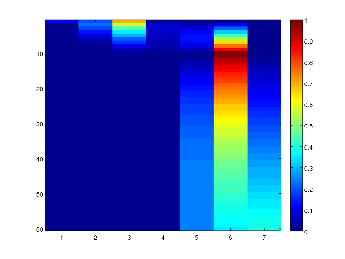
As in the unconditional case, the node marginals reveal a lot more of the
structure in our model than the optimal decoding. For example, we
see that people who are in academia after 10 years had a ~0.70 probability of
starting in the 'Grad School' (3) state, which is very different than the 0.30
probability we assumed of a random CS grad. We also see that the student has
zero probability of being in the 'Industry' (2) or 'Video Games' (1) states in their
9th year (or of being deceased before their 10th year), since these have zero
probability of transitioning to 'Academia' in the 10th year. Finally, we see
that being in Academia in our second year only has a probability of around
~0.10, despite being part of the conditionally most likely sequence.
To generate samples from the model to see what those working in Academia do
after their 10th year, we use the conditional sampling function:
samples = UGM_Sample_Conditional(nodePot,edgePot,edgeStruct,clamped,@UGM_Sample_Tree)
imagesc(samples');
xlabel('Year after graduation');
ylabel('Graduate');
colorbar
An example of 100 conditional samples from the model is:
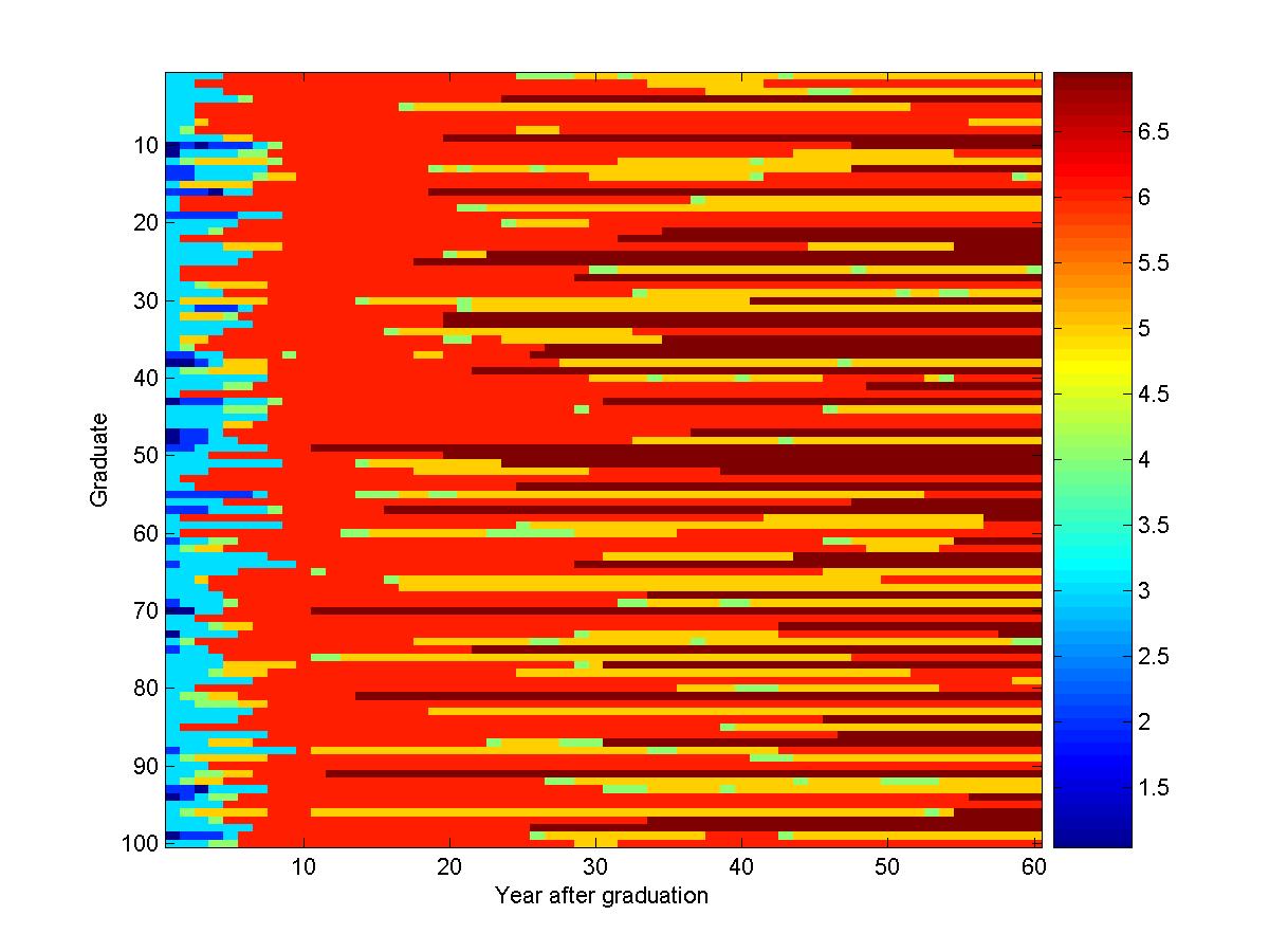
Of course, this looks very different than the unconditional samples of the
model we generated in the second demo.
We want to know what happens in the water system when the source node is in the
'very unsafe' (4) state. We first make the water system UGM:
load('waterSystem.mat'); % Loads adj
nNodes = length(adj);
nStates = 4;
edgeStruct = UGM_makeEdgeStruct(adj,nStates);
source = 4;
nodePot = ones(nNodes,nStates);
nodePot(source,:) = [.9 .09 .009 .001];
transition = [  0.9890    0.0099    0.0010    0.0001
    0.1309    0.8618    0.0066    0.0007
    0.0420    0.0841    0.8682    0.0057
    0.0667    0.0333    0.1667    0.7333];
colored = zeros(nNodes,1);
colored(source) = 1;
done = 0;
edgePot = zeros(nStates,nStates,edgeStruct.nEdges);
while ~done
    done = 1;
    colored_old = colored;

    for e = 1:edgeStruct.nEdges
        if sum(colored_old(edgeStruct.edgeEnds(e,:))) == 1
            % Determine direction of edge and color nodes
            if colored(edgeStruct.edgeEnds(e,1)) == 1
                edgePot(:,:,e) = transition;
            else
                edgePot(:,:,e) = transition';
            end
            colored(edgeStruct.edgeEnds(e,:)) = 1;
            done = 0;
        end
    end
end
We now make the clamped vector, clamping the source node (4) to the 'very
unsafe' state (4):
clamped = zeros(nNodes,1);
clamped(4) = 4;
We can now perform decoding/inference/sampling with the source node in this state
using:
optimalDecoding = UGM_Decode_Conditional(nodePot,edgePot,edgeStruct,clamped,@UGM_Decode_Tree)
[nodeBel,edgeBel,logZ] = UGM_Infer_Conditional(nodePot,edgePot,edgeStruct,clamped,@UGM_Infer_Tree);
nodeBel
samples = UGM_Sample_Conditional(nodePot,edgePot,edgeStruct,clamped,@UGM_Sample_Tree)
imagesc(samples');
xlabel('Node');
ylabel('Sample');
colorbar
The optimal conditional decoding reveals that the most likely configuration of the
remaining parts of the water system are all 'very safe'. However, the
conditional marginals reveal a different story:
nodeBel =

    0.3702    0.1842    0.3254    0.1202
    0.4119    0.1938    0.3041    0.0902
    0.5576    0.2008    0.2112    0.0305
         0         0         0    1.0000
    0.2320    0.1284    0.3469    0.2928
    0.5576    0.2008    0.2112    0.0305
    0.4515    0.1997    0.2808    0.0680
    0.2803    0.1518    0.3510    0.2168
    0.1262    0.0678    0.2673    0.5387
    0.2803    0.1518    0.3510    0.2168
    0.5576    0.2008    0.2112    0.0305
    0.4890    0.2024    0.2569    0.0517
    0.7133    0.1681    0.1106    0.0081
    0.4119    0.1938    0.3041    0.0902
    0.2803    0.1518    0.3510    0.2168
    0.1809    0.1001    0.3224    0.3966
    0.2320    0.1284    0.3469    0.2928
    0.3702    0.1842    0.3254    0.1202
    0.5244    0.2026    0.2335    0.0396
    0.4515    0.1997    0.2808    0.0680
    0.6693    0.1811    0.1377    0.0120
    0.5244    0.2026    0.2335    0.0396
    0.2803    0.1518    0.3510    0.2168
    0.3702    0.1842    0.3254    0.1202
    0.3263    0.1704    0.3422    0.1611
    0.5886    0.1973    0.1903    0.0238
    0.5576    0.2008    0.2112    0.0305
    0.5576    0.2008    0.2112    0.0305
    0.4515    0.1997    0.2808    0.0680
    0.5576    0.2008    0.2112    0.0305
    0.4515    0.1997    0.2808    0.0680
    0.4119    0.1938    0.3041    0.0902
    0.4515    0.1997    0.2808    0.0680
    0.4890    0.2024    0.2569    0.0517
    0.6922    0.1747    0.1234    0.0098
    0.5886    0.1973    0.1903    0.0238
    0.4890    0.2024    0.2569    0.0517
    0.2320    0.1284    0.3469    0.2928
    0.4515    0.1997    0.2808    0.0680
    0.4515    0.1997    0.2808    0.0680
    0.6175    0.1927    0.1711    0.0187
    0.2320    0.1284    0.3469    0.2928
    0.6175    0.1927    0.1711    0.0187
    0.3263    0.1704    0.3422    0.1611
    0.6693    0.1811    0.1377    0.0120
    0.5244    0.2026    0.2335    0.0396
    0.5886    0.1973    0.1903    0.0238
    0.4515    0.1997    0.2808    0.0680
    0.3263    0.1704    0.3422    0.1611
    0.6175    0.1927    0.1711    0.0187
    0.2320    0.1284    0.3469    0.2928
    0.1809    0.1001    0.3224    0.3966
    0.6693    0.1811    0.1377    0.0120
    0.4515    0.1997    0.2808    0.0680
    0.5886    0.1973    0.1903    0.0238
    0.6922    0.1747    0.1234    0.0098
    0.1809    0.1001    0.3224    0.3966
    0.3702    0.1842    0.3254    0.1202
    0.5886    0.1973    0.1903    0.0238
    0.5886    0.1973    0.1903    0.0238
    0.4119    0.1938    0.3041    0.0902
    0.3263    0.1704    0.3422    0.1611
    0.5886    0.1973    0.1903    0.0238
    0.2320    0.1284    0.3469    0.2928
    0.6444    0.1872    0.1535    0.0149
    0.4515    0.1997    0.2808    0.0680
    0.1809    0.1001    0.3224    0.3966
    0.6175    0.1927    0.1711    0.0187
    0.6693    0.1811    0.1377    0.0120
    0.0667    0.0333    0.1667    0.7333
    0.4515    0.1997    0.2808    0.0680
    0.3702    0.1842    0.3254    0.1202
    0.5244    0.2026    0.2335    0.0396
    0.4890    0.2024    0.2569    0.0517
    0.2803    0.1518    0.3510    0.2168
    0.2320    0.1284    0.3469    0.2928
    0.4515    0.1997    0.2808    0.0680
    0.4890    0.2024    0.2569    0.0517
    0.3263    0.1704    0.3422    0.1611
    0.6175    0.1927    0.1711    0.0187
    0.6444    0.1872    0.1535    0.0149
    0.4515    0.1997    0.2808    0.0680
    0.4119    0.1938    0.3041    0.0902
    0.5576    0.2008    0.2112    0.0305
    0.4890    0.2024    0.2569    0.0517
    0.1809    0.1001    0.3224    0.3966
    0.2803    0.1518    0.3510    0.2168
    0.3263    0.1704    0.3422    0.1611
    0.5886    0.1973    0.1903    0.0238
    0.4890    0.2024    0.2569    0.0517
    0.2803    0.1518    0.3510    0.2168
    0.5576    0.2008    0.2112    0.0305
    0.4119    0.1938    0.3041    0.0902
    0.3702    0.1842    0.3254    0.1202
    0.4119    0.1938    0.3041    0.0902
    0.2320    0.1284    0.3469    0.2928
    0.1262    0.0678    0.2673    0.5387
    0.5886    0.1973    0.1903    0.0238
    0.4890    0.2024    0.2569    0.0517
    0.4890    0.2024    0.2569    0.0517
The probabilities of the non-source nodes being 'very unsafe' ranges from ~0.01 to ~0.73,
indicating that (as is often the case) the optimal decoding is misleading. An
example of 100 conditional samples of the model is:
The Multiple Source Water Turbidity Problem
We now consider a slightly more complicated variant of the water turbidity
problem. In it, we use a graph containing 400 nodes, with 10 source nodes:
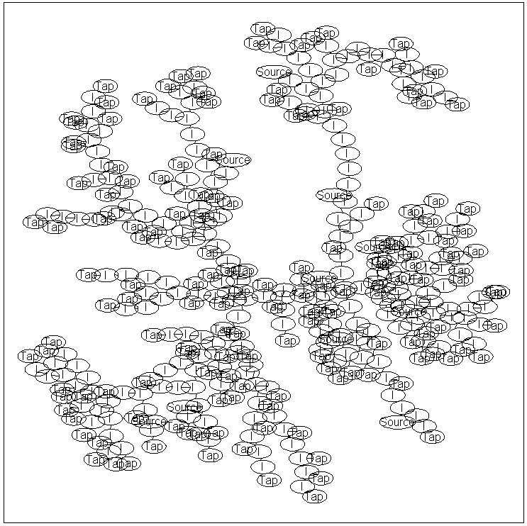
We can use conditional queries in this graph to answer questions like: if node
300 takes the state '4', which sources are likely to be at higher levels.
We make the edgeStruct and nodePot as before (the source nodes are 1, 6, 7, 8,
11, 12, 15, 17, 19, and 20):
load('waterSystem2.mat'); % Loads adj
nNodes = length(adj);
nStates = 4;
edgeStruct = UGM_makeEdgeStruct(adj,nStates);
source = [1 6 7 8 11 12 15 17 19 20];
nodePot = ones(nNodes,nStates);
nodePot(source,:) = repmat([.9 .09 .009 .001],length(source),1);
Because we have non-unit values for more than one node, we can no longer
interpret the node and edge potentials in the model as probabilities. That is,
the node marginals of the source nodes will no longer be the same as the node
potentials.
To make
the edge potentials, we use:
transition = [  0.9890    0.0099    0.0010    0.0001
    0.1309    0.8618    0.0066    0.0007
    0.0420    0.0841    0.8682    0.0057
    0.0667    0.0333    0.1667    0.7333];
colored = zeros(nNodes,1);
colored(source) = 1;
coloredEdges = zeros(edgeStruct.nEdges,1);
done = 0;
edgePot = zeros(nStates,nStates,edgeStruct.nEdges);
while ~done
    done = 1;
    colored_old = colored;

    for e = 1:edgeStruct.nEdges
        if sum(colored_old(edgeStruct.edgeEnds(e,:))) == 1
            % Determine direction of edge and color nodes
            if colored(edgeStruct.edgeEnds(e,1)) == 1
                edgePot(:,:,e) = transition;
            else
                edgePot(:,:,e) = transition';
            end
            colored(edgeStruct.edgeEnds(e,:)) = 1;
                        coloredEdges(e) = 1;
            done = 0;
        end
    end
end
for e = 1:edgeStruct.nEdges
   if coloredEdges(e) == 0
      edgePot(:,:,e) = (transition+transition')/2;
   end
end
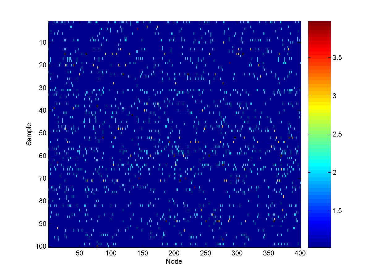
We first compute the unconditional marginals and generate some unconditional
samples. The unconditional marginals for the first 20 nodes are:
[nodeBel,edgeBel,logZ] = UGM_Infer_Tree(nodePot,edgePot,edgeStruct);

nodeBel(1:20,:)

ans =

    0.9511    0.0464    0.0022    0.0003
    0.9579    0.0389    0.0029    0.0003
    0.9805    0.0189    0.0006    0.0001
    0.9362    0.0565    0.0068    0.0005
    0.9489    0.0477    0.0030    0.0003
    0.9703    0.0286    0.0010    0.0002
    0.9467    0.0504    0.0025    0.0003
    0.9836    0.0159    0.0005    0.0001
    0.9787    0.0191    0.0020    0.0002
    0.9546    0.0424    0.0027    0.0003
    0.9430    0.0539    0.0028    0.0003
    0.9640    0.0344    0.0014    0.0002
    0.9498    0.0462    0.0037    0.0003
    0.9322    0.0597    0.0076    0.0006
    0.9391    0.0573    0.0032    0.0004
    0.9572    0.0380    0.0044    0.0004
    0.9297    0.0657    0.0041    0.0005
    0.9283    0.0627    0.0084    0.0006
    0.9652    0.0335    0.0011    0.0002
    0.9640    0.0344    0.0014    0.0002
As we discussed above, the node marginals of the sources are no longer equal to
the node potentials.
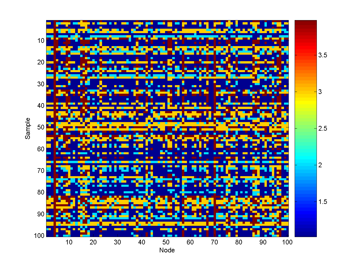
100 samples from the unconditional model look like:
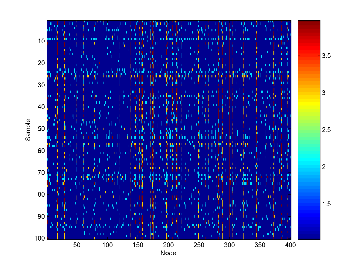
We now want to think about answering queries about the sources, given the
values of some other nodes. We will consider conditioning on node 300 taking
the value 4, and will compute conditional samples from the model as well as the marginals of the source nodes:
clamped = zeros(nNodes,1);
clamped(300) = 4;
samples = UGM_Sample_Conditional(nodePot,edgePot,edgeStruct,clamped,@UGM_Sample_Tree);
figure(4);
imagesc(samples');
xlabel('Node');
ylabel('Sample');
colorbar
[nodeBel,edgeBel,logZ] = UGM_Infer_Conditional(nodePot,edgePot,edgeStruct,clamped,@UGM_Infer_Tree);
nodeBel(source,:)

ans =

    0.9509    0.0466    0.0022    0.0003
    0.9703    0.0286    0.0010    0.0002
    0.9467    0.0505    0.0025    0.0003
    0.9836    0.0159    0.0005    0.0001
    0.9430    0.0539    0.0028    0.0003
    0.9640    0.0344    0.0014    0.0002
    0.9391    0.0573    0.0032    0.0004
    0.8450    0.1144    0.0280    0.0126
    0.9652    0.0335    0.0011    0.0002
    0.9640    0.0344    0.0014    0.0002
From these conditional node marginals, we see that (among the sources) the 3rd
last source (corresponding to node 17) is the
most likely source to also be at a very unsafe level. Conditional samples from
the model look like:
PREVIOUS DEMO NEXT DEMO
Mark Schmidt > Software > UGM > Condition Demo