TrainCRF UGM Demo

The MRF model we used in the last demo was fairly naive, and it can be improved in various ways. As one example, in this demo we will take into account the month of the year. One way to do this would be add a 12-state 'month' variable to the model that is connected to every node. We could then do parameter estimation in the model by cutset conditioning (i.e. we condition on the month variable so that the remaining variables form a chain). We could subsequently do conditional decoding/inference/sampling in the model, where we condition on the month.

If we are only interested in conditional queries, then a conditional random field (CRF) might be a better option. In CRFs, we have two types of variables: (i) the 'features' (also known as 'covariates') X are treated as fixed non-random variables, and (ii) the 'labels' y are treated as random variables in a UGM, where the parameters of the UGM depend on the features. In our case, the 'labels' will be the 28 variables representing days of the month, and the features will consist of a 'bias' feature and a set of indicator variables that will represent the month. That is, each possible value that the features can take leads to a different UGM model of the labels.

Vancouver Rain Data, with Months

In addition to the matrix of binarized daily precipitation values, the file 'rain.mat' also contains a vector months that contains a number in the range 1-12, representing the month of the year. We might hope to get a better model by using this data, since common sense would indicate that it is more likely to rain in December than July. Of course, since we have the relevant data we don't need to just assume that our common sense is correct; we can use the data to find a good way to incorporate the month information. In particular, we are going to use a CRF where the months are used to define the features, and the binarized daily precipitation values represent the labels. As before, the first step will be loading the data and making the edgeStruct: load rain.mat y = int32(X+1); [nInstances,nNodes] = size(y); nStates = max(y); adj = zeros(nNodes); for i = 1:nNodes-1 adj(i,i+1) = 1; end adj = adj+adj'; edgeStruct = UGM_makeEdgeStruct(adj,nStates); maxState = max(nStates);
Note that we have used y to denote the samples of the random variables in this demo, since X is typically used to denote the features in a CRF model.

Representing the Features

To train CRFs, we need to make the arrays Xnode and Xedge. Xnode represents features that affect the node potentials, while Xedge represents features that affect the edge potentials. Note that unlike the labels y, UGM assumes that Xnode and Xedge are stored in Matlab's default double format.

For our first CRF model, we will only use a single 'bias' feature for the node and edge potentials. A 'bias' feature is a feature that always set to one, and it is included to reflect any effects on the states that are independent of the features. MRFs correspond to the special case where we only have a bias variable. In general, the features in CRFs can be arbitrary real-valued numbers and thus we do not necessarily need to include a bias variable. However, unless the states are perfectly balanced in the training data it usually makes sense to include a bias variable. After training this simple model (and verifying that it gives the same results as the previous demo), we will move on to using node and edge features that incorporate the month information to give a better model.

If our CRF has nInstances (conditional) samples of nNodes random variables, and we have nNodeFeatures features for each node, then the Xnode variable will be a nInstances by nNodeFeatures by nNodes array, each element containing the relevant feature for the appropriate node in the particular instance. Therefore, for the simple case where we only have a single unit-valued feature, we would make Xnode as follows:

Xnode = ones(nInstances,1,nNodes);

Similarly, the Xedge variable will be a nInstances by nEdgeFeatures by nEdges array. To make the simple unit-valued edge features we use: nEdges = edgeStruct.nEdges; Xedge = ones(nInstances,1,nEdges);

Making the nodeMap and edgeMap

For training CRFs, the nodeMap and edgeMap have an extra dimension since they must take into account how the features are parameterized. As in the case of MRFs, UGM uses a log-linear parameterization of CRFs. This again allows us to again state maximum likelihood estimation as a convex optimization problem. In particular, for training example i UGM uses the following convention:

We set nodePot(n,s) = exp(sum_f w(nodeMap(n,s,f))*Xnode(i,f,n)).
We set edgePot(s1,s2,e)= exp(sum_f w(edgeMap(s1,s2,e,f)*Xedge(i,f,e)).

The following image (due to Yu Zhou) illustrates how the nodeMap/edgeMap interact with the Xnode/Xedge and w to give the potentials:

Maximum Likelihood Training of Log-Linear Conditionals Random Fields

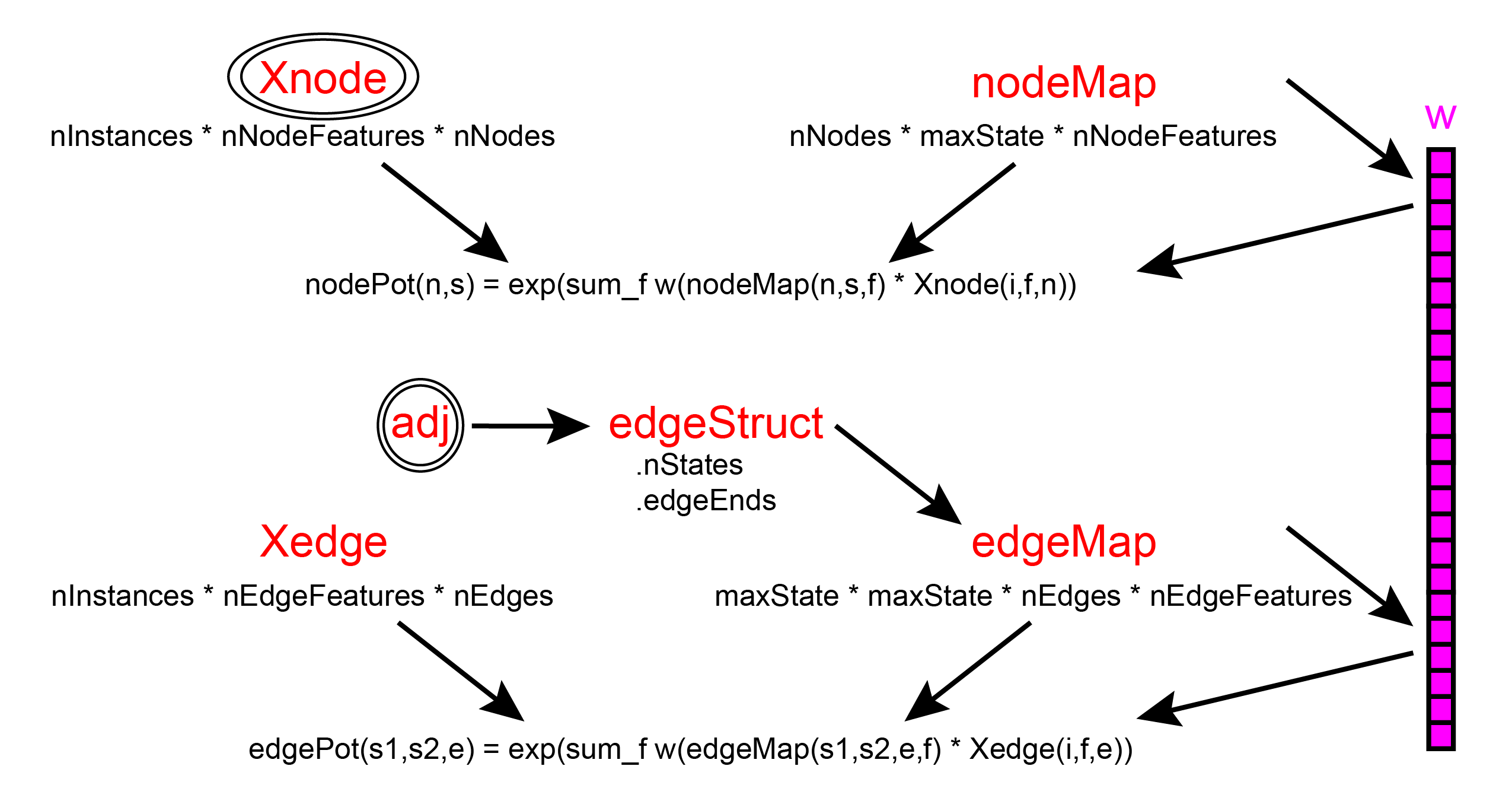
Training CRFs with UGM is very similar to the case of MRFs. The main differences are that the nodeMap and edgeMap have the extra dimension that takes into account how each feature is parameterized, and that we pass the features as opposed to the sufficient statistics to the negative log-likelihood function.

In the case where have only one feature, we don't use the extra dimension of the nodeMap and edgeMap variables so they can be constructed as before:

nodeMap = zeros(nNodes,maxState,'int32');
nodeMap(:,1) = 1;

edgeMap = zeros(maxState,maxState,nEdges,'int32');
edgeMap(1,1,:) = 2;
edgeMap(2,1,:) = 3;
edgeMap(1,2,:) = 4;

To initialize the parameters, we proceed as before: nParams = max([nodeMap(:);edgeMap(:)]); w = zeros(nParams,1);
We will again consider minimizing the negative log-likelihood in order to maximize the likelihood. The negative log-likelihood (and its) gradient are computed by UGM_CRF_NLL. With log-linear CRFs, the negative log-likelihood is still differentiable and jointly convex in the node and edge parameters, so we can again computes its optimal value using minFunc. The negative log-likelihood for CRFs takes similar arguments to the MRF case, but we pass in the features instead of sufficient statistics: w = minFunc(@UGM_CRF_NLL,randn(size(w)),[],Xnode,Xedge,y,nodeMap,edgeMap,edgeStruct,@UGM_Infer_Chain) Iteration FunEvals Step Length Function Val Opt Cond 1 2 3.19683e-05 2.83032e+04 9.07391e+03 2 3 1.00000e+00 2.42379e+04 7.08784e+03 3 4 1.00000e+00 2.13785e+04 3.39832e+03 4 5 1.00000e+00 1.95148e+04 2.92734e+03 5 6 1.00000e+00 1.79881e+04 5.36254e+02 6 7 1.00000e+00 1.79304e+04 6.91542e+02 7 8 1.00000e+00 1.79114e+04 1.85252e+02 8 10 1.00000e+01 1.78885e+04 7.54564e+02 9 11 1.00000e+00 1.78582e+04 6.71792e+02 10 12 1.00000e+00 1.78035e+04 5.24928e+01 11 13 1.00000e+00 1.78032e+04 1.59129e+01 12 14 1.00000e+00 1.78031e+04 2.55631e+01 13 15 1.00000e+00 1.78028e+04 5.82554e+01 14 16 1.00000e+00 1.78021e+04 9.26333e+01 15 17 1.00000e+00 1.78007e+04 1.23620e+02 16 18 1.00000e+00 1.77990e+04 1.09300e+02 17 19 1.00000e+00 1.77979e+04 3.57499e+01 18 20 1.00000e+00 1.77977e+04 4.54387e+00 19 21 1.00000e+00 1.77977e+04 1.01720e-01 20 22 1.00000e+00 1.77977e+04 3.55628e-02 21 23 1.00000e+00 1.77977e+04 1.99919e-03 Directional Derivative below progTol w = 0.5968 -0.4499 -1.1506 -1.0029
As we expected, this degenerate CRF gives us exactly the model we had in the last MRF demo. However, note that training was a bit slower. This is because each instance in a CRF is potentially a different UGM, so the loss function needs to call inferFunc for every sample.

In CRFs, the potentials depend on the features. So to make a set of potentials, we need to choose a set of features. The function UGM_CRF_makePotentials takes a training instance number and returns the corresponding potentials. For example, to return the potentials associated with the first training example we would use

instance = 1;
[nodePot,edgePot] = UGM_CRF_makePotentials(w,Xnode,Xedge,nodeMap,edgeMap,edgeStruct,instance);
nodePot(1,:)
edgePot(:,:,1)

ans =

    1.8163    1.0000


ans =

    0.6377    0.3668
    0.3165    1.0000

As expected, these are the same potentials we had before.

Using Node Features

We now want to make a set of node features that incorporate the months of the year. Since the potentials will be formed by exponentiating a linear function of the features, we will represent the months as a set of 12 binary indicator variables: nFeatures = 12; Xnode = zeros(nInstances,nFeatures,nNodes); for m = 1:nFeatures Xnode(months==m,m,:) = 1; end
For example, Xnode(3,4,1) is set to 1 while Xnode(3,[1:3 5:12],1) is 0 because the month variable for the third sample is set to 4 (representing April). We will also want a bias in the model (since we expect there to be some baseline probability of rain that is independent of the month), so we add a feature that is always set to 1:

Xnode = [ones(nInstances,1,nNodes) Xnode];
nNodeFeatures = size(Xnode,2);

We now make the nNodes by maxState by nNodeFeatures nodeMap, which lets UGM know which features multiplied together and then added and exponentiated for each variable. In our case, all variables will use all 13 features but share the same parameters, so we use: nodeMap = zeros(nNodes,maxState,nNodeFeatures,'int32'); for f = 1:nNodeFeatures nodeMap(:,1,f) = f; end
We also need to update the edgeMap, so that the nodeMap and edgeMap numbers don't overlap (it rarely makes sense to share node and edge parameters): edgeMap = zeros(maxState,maxState,nEdges,'int32'); edgeMap(1,1,:) = nNodeFeatures+1; edgeMap(2,1,:) = nNodeFeatures+2; edgeMap(1,2,:) = nNodeFeatures+3;
With the updated nodeMap and edgeMap, training proceeds exactly as before:

nParams = max([nodeMap(:);edgeMap(:)]);
w = zeros(nParams,1);
w = minFunc(@UGM_CRF_NLL,w,[],Xnode,Xedge,y,nodeMap,edgeMap,edgeStruct,@UGM_Infer_Chain)

 Iteration   FunEvals     Step Length    Function Val        Opt Cond
         1          2     5.50957e-05     1.87895e+04     1.71063e+03
         2          3     1.00000e+00     1.83557e+04     1.71053e+03
         3          4     1.00000e+00     1.76199e+04     3.06222e+03
         4          5     1.00000e+00     1.73411e+04     7.91786e+02
         5          6     1.00000e+00     1.73097e+04     2.19752e+02
         6          7     1.00000e+00     1.72916e+04     2.66328e+02
         7          8     1.00000e+00     1.72552e+04     5.10685e+02
         8          9     1.00000e+00     1.72132e+04     4.40088e+02
         9         10     1.00000e+00     1.71942e+04     8.79763e+01
        10         11     1.00000e+00     1.71925e+04     5.99177e+01
        11         12     1.00000e+00     1.71918e+04     8.47407e+01
        12         13     1.00000e+00     1.71893e+04     1.21715e+02
        13         14     1.00000e+00     1.71855e+04     1.22600e+02
        14         15     1.00000e+00     1.71756e+04     2.08079e+02
        15         16     1.00000e+00     1.71695e+04     1.12069e+02
        16         17     1.00000e+00     1.71670e+04     1.95784e+01
        17         18     1.00000e+00     1.71668e+04     1.46669e+01
        18         19     1.00000e+00     1.71665e+04     1.99287e+01
        19         20     1.00000e+00     1.71661e+04     1.94539e+01
        20         21     1.00000e+00     1.71659e+04     3.94953e+00
        21         22     1.00000e+00     1.71658e+04     1.08766e+00
        22         23     1.00000e+00     1.71658e+04     1.80154e-01
        23         24     1.00000e+00     1.71658e+04     8.30007e-02
        24         25     1.00000e+00     1.71658e+04     2.70300e-02
        25         26     1.00000e+00     1.71658e+04     2.17654e-03
        26         27     1.00000e+00     1.71658e+04     2.90511e-04
Directional Derivative below progTol

w =

    0.5662
   -0.3639
   -0.1622
   -0.0970
    0.0183
    0.1848
    0.2275
    0.6032
    0.6072
    0.3090
   -0.0487
   -0.3435
   -0.3684
   -0.4218
   -1.0356
   -0.8798

As expected, conditioning on the month information leads to a better fit. In fact, the improvement between the likelihood of the CRF model and the MRF model is much bigger than the improvement that we obtained by using more expressive edge potentials in the previous demo.

Using Edge Features

In the above CRF model, the node potentials depend on the features but the edges do not. That is, the model doesn't take into account that the months could also affect the chances of transitioning from/to rain. To make our edge potentials also depend on the months, we will make a new Xedge that incorporates month information. One way to make the edge features given the node features is with the function UGM_makeEdgeFeatures. The function looks at the node features for each node on the edge, and does one of two things: (i) if the feature is 'shared' then it uses the node feature from the first node (as defined by the edgeEnds structure), (ii) otherwise, it uses the features from both edge ends as features. In our case, it makes sense to use the 'shared' case for all the node features, since all nodes have the same features (for a given training example): sharedFeatures = ones(13,1); Xedge = UGM_makeEdgeFeatures(Xnode,edgeStruct.edgeEnds,sharedFeatures); nEdgeFeatures = size(Xedge,2);
We now make the maxState by maxState by nEdges by nEdgeFeatures edgeMap: edgeMap = zeros(maxState,maxState,nEdges,nEdgeFeatures,'int32'); for edgeFeat = 1:nEdgeFeatures for s1 = 1:2 for s2 = 1:2 f = f+1; edgeMap(s1,s2,:,edgeFeat) = f; end end end
With the updated Xedge and edgeMap, we proceed as before: nParams = max([nodeMap(:);edgeMap(:)]); w = zeros(nParams,1); w = minFunc(@UGM_CRF_NLL,w,[],Xnode,Xedge,y,nodeMap,edgeMap,edgeStruct,@UGM_Infer_Chain) Iteration FunEvals Step Length Function Val Opt Cond 1 2 2.99873e-05 1.90436e+04 2.55653e+03 2 3 1.00000e+00 1.76400e+04 2.34032e+03 3 4 1.00000e+00 1.72738e+04 5.65236e+02 4 5 1.00000e+00 1.72512e+04 1.96187e+02 5 6 1.00000e+00 1.72162e+04 4.73894e+02 6 7 1.00000e+00 1.71816e+04 4.29853e+02 7 8 1.00000e+00 1.71676e+04 9.36649e+01 8 9 1.00000e+00 1.71657e+04 8.10747e+01 9 10 1.00000e+00 1.71645e+04 1.35856e+02 10 11 1.00000e+00 1.71614e+04 2.06251e+02 11 12 1.00000e+00 1.71575e+04 2.03290e+02 12 13 1.00000e+00 1.71545e+04 1.92202e+02 13 14 1.00000e+00 1.71492e+04 4.64233e+01 14 15 1.00000e+00 1.71475e+04 7.23352e+01 15 16 1.00000e+00 1.71461e+04 1.38713e+02 16 17 1.00000e+00 1.71440e+04 1.75369e+02 17 18 1.00000e+00 1.71414e+04 1.30053e+02 18 19 1.00000e+00 1.71397e+04 2.82008e+01 19 20 1.00000e+00 1.71390e+04 5.28906e+01 20 21 1.00000e+00 1.71386e+04 9.04927e+01 21 22 1.00000e+00 1.71378e+04 1.27399e+02 22 23 1.00000e+00 1.71366e+04 1.29590e+02 23 24 1.00000e+00 1.71350e+04 8.02345e+01 24 25 1.00000e+00 1.71338e+04 2.14189e+01 25 26 1.00000e+00 1.71328e+04 6.68356e+01 26 27 1.00000e+00 1.71323e+04 8.78730e+01 27 28 1.00000e+00 1.71310e+04 1.01143e+02 28 29 1.00000e+00 1.71288e+04 9.07294e+01 29 30 1.00000e+00 1.71255e+04 2.70413e+01 30 31 1.00000e+00 1.71234e+04 2.33995e+01 31 32 1.00000e+00 1.71226e+04 3.42237e+01 32 33 1.00000e+00 1.71223e+04 2.23663e+01 33 34 1.00000e+00 1.71220e+04 5.62033e+00 34 35 1.00000e+00 1.71220e+04 1.69890e+01 35 36 1.00000e+00 1.71218e+04 3.02428e+01 36 37 1.00000e+00 1.71217e+04 2.99272e+01 37 38 1.00000e+00 1.71211e+04 3.03047e+01 38 39 1.00000e+00 1.71202e+04 4.71917e+01 39 40 1.00000e+00 1.71186e+04 1.46650e+01 40 41 1.00000e+00 1.71177e+04 1.22074e+01 41 42 1.00000e+00 1.71172e+04 8.57846e+00 42 43 1.00000e+00 1.71171e+04 1.83532e+01 43 44 1.00000e+00 1.71169e+04 6.84019e+00 44 45 1.00000e+00 1.71168e+04 2.20643e+00 45 46 1.00000e+00 1.71167e+04 3.27873e+00 46 47 1.00000e+00 1.71167e+04 1.20115e+00 47 48 1.00000e+00 1.71167e+04 2.22905e+00 48 49 1.00000e+00 1.71167e+04 5.42830e+00 49 50 1.00000e+00 1.71167e+04 9.00362e+00 50 51 1.00000e+00 1.71166e+04 9.82641e+00 51 52 1.00000e+00 1.71165e+04 1.27488e+01 52 54 4.72543e-01 1.71165e+04 8.33743e+00 53 55 1.00000e+00 1.71164e+04 4.89122e+00 54 56 1.00000e+00 1.71164e+04 6.44481e-01 55 57 1.00000e+00 1.71164e+04 5.46661e-01 56 58 1.00000e+00 1.71164e+04 1.36614e+00 57 59 1.00000e+00 1.71164e+04 2.46083e+00 58 60 1.00000e+00 1.71164e+04 2.87980e+00 59 61 1.00000e+00 1.71164e+04 2.40811e+00 60 62 1.00000e+00 1.71164e+04 3.14707e+00 61 63 1.00000e+00 1.71163e+04 2.01836e+00 62 64 1.00000e+00 1.71163e+04 2.46767e+00 63 65 1.00000e+00 1.71163e+04 2.55408e+00 64 67 4.04260e-01 1.71163e+04 1.56098e+00 65 68 1.00000e+00 1.71163e+04 3.12589e-01 66 69 1.00000e+00 1.71163e+04 2.40309e-01 67 70 1.00000e+00 1.71163e+04 3.51821e-01 68 71 1.00000e+00 1.71163e+04 6.98811e-01 69 72 1.00000e+00 1.71163e+04 1.25232e+00 70 73 1.00000e+00 1.71163e+04 1.74637e+00 71 74 1.00000e+00 1.71163e+04 1.82086e+00 72 76 4.32633e-01 1.71163e+04 1.38697e+00 73 77 1.00000e+00 1.71163e+04 5.39311e-01 74 78 1.00000e+00 1.71163e+04 1.37194e-01 75 79 1.00000e+00 1.71163e+04 4.85571e-02 76 80 1.00000e+00 1.71163e+04 3.82990e-02 77 81 1.00000e+00 1.71163e+04 2.54560e-02 78 82 1.00000e+00 1.71163e+04 4.69787e-02 79 83 1.00000e+00 1.71163e+04 8.66219e-02 80 84 1.00000e+00 1.71163e+04 1.35306e-01 81 85 1.00000e+00 1.71163e+04 8.59283e-02 82 86 1.00000e+00 1.71163e+04 1.67533e-01 83 87 1.00000e+00 1.71163e+04 1.30266e-02 84 88 1.00000e+00 1.71163e+04 1.01122e-02 85 90 1.00000e+01 1.71163e+04 2.79276e-02 86 91 1.00000e+00 1.71163e+04 2.97327e-02 87 92 1.00000e+00 1.71163e+04 4.27361e-02 88 93 1.00000e+00 1.71163e+04 2.10481e-02 89 94 1.00000e+00 1.71163e+04 4.44461e-03 90 95 1.00000e+00 1.71163e+04 4.32501e-03 91 96 1.00000e+00 1.71163e+04 5.82381e-03 92 97 1.00000e+00 1.71163e+04 8.82892e-03 93 98 1.00000e+00 1.71163e+04 1.32052e-02 94 99 1.00000e+00 1.71163e+04 1.62503e-02 95 100 1.00000e+00 1.71163e+04 1.40167e-02 96 101 1.00000e+00 1.71163e+04 3.80935e-03 97 102 1.00000e+00 1.71163e+04 2.07595e-03 98 103 1.00000e+00 1.71163e+04 5.51650e-04 99 104 1.00000e+00 1.71163e+04 8.77187e-04 100 105 1.00000e+00 1.71163e+04 1.56245e-03 101 106 1.00000e+00 1.71163e+04 2.42554e-03 102 107 1.00000e+00 1.71163e+04 2.95997e-03 103 108 1.00000e+00 1.71163e+04 2.76296e-03 104 110 2.44377e-01 1.71163e+04 4.14080e-03 105 111 1.00000e+00 1.71163e+04 2.18171e-03 106 112 1.00000e+00 1.71163e+04 4.59363e-04 107 113 1.00000e+00 1.71163e+04 6.28469e-04 108 114 1.00000e+00 1.71163e+04 1.78548e-03 109 115 1.00000e+00 1.71163e+04 3.70297e-03 110 116 1.00000e+00 1.71163e+04 5.67089e-03 111 117 1.00000e+00 1.71163e+04 6.25322e-03 112 119 2.20033e-02 1.71163e+04 6.23359e-03 113 120 1.00000e+00 1.71163e+04 3.85092e-03 114 121 1.00000e+00 1.71163e+04 8.83878e-04 Directional Derivative below progTol w = 0.6249 -0.4527 -0.6101 -0.3241 0.4608 -0.3367 0.5082 1.0738 1.5220 0.1323 0.1217 -0.2454 -1.2248 0.1201 -0.2996 -0.4049 0.5844 0.0663 -0.1287 0.0724 -0.0100 0.2604 0.1159 -0.1940 -0.1823 0.1009 0.0248 -0.0077 -0.1180 -0.2939 -0.0535 0.2040 0.1434 0.2591 0.0059 0.0167 -0.2816 -0.1454 -0.1638 0.1644 0.1448 -0.1869 -0.7289 0.4606 0.4552 -0.4338 0.0364 -0.2204 0.6178 0.1368 -0.0791 -0.0796 0.0220 -0.0843 0.3841 -0.4049 0.1051 -0.0467 0.3905 -0.4187 0.0749 0.4876 -0.1031 0.0023 -0.3868
Although not as drastic as the improvement obtained by adding the node features, adding the edge features leads to a further improvement in the training set negative log-likelihood.

The function UGM_makeEdgeFeatures only represents one possible way to construct the edge features (by simply using the corresponding node features). Provided that Xedge has the right size and is real-valued, you can use any edge features you like. For example, when using continuous node features, using edge features that depend on the differences between node features might make sense. You could also consider edge features that do not depend on the node features.

Using the Estimated Parameters

As an example of using the learned model, we will generate samples when the binary 'December' feature is on. The first example of a December in the training data is instance 11, so we can generate samples of December using: i = 11; [nodePot,edgePot] = UGM_CRF_makePotentials(w,Xnode,Xedge,nodeMap,edgeMap,edgeStruct,i); samples = UGM_Sample_Chain(nodePot,edgePot,edgeStruct);
Below is an example:

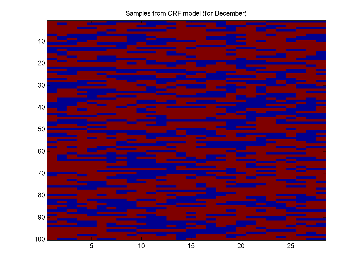
As expected, when we let the model know that it should generate samples of December, it predicts a lot more rain (red).

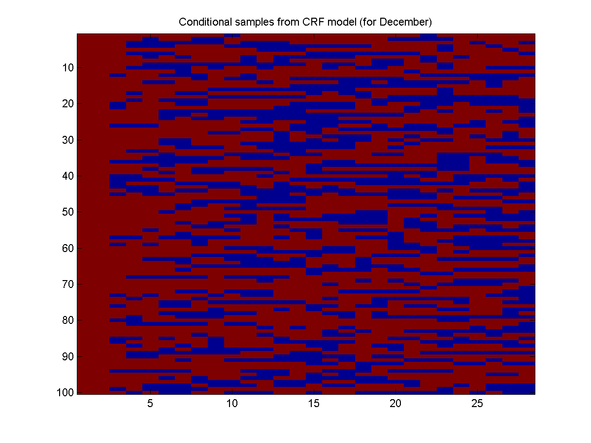
Next, we will repeat our scenario from the previous demo where we want to know what the rest of the month will look like given that it rained for the first two days. However, we will now ask the question conditioned on the information that the month is Decmber:

clamped = zeros(nNodes,1);
clamped(1:2) = 2;
condSamples = UGM_Sample_Conditional(nodePot,edgePot,edgeStruct,clamped,@UGM_Sample_Chain);

Here is the result:

With a trained CRF, we don't necessarily have to use the Xnode and Xedge from the training data. In principle, we could make up whatever node and edge features we want, and see what the model predicts for that scenario. For example, instead of looking for a training example in July, we could just make the relevant node and edge features. Below, we make the node/edge features for July, and then generate 100 samples of July (note that UGM_CRF_makePotentials makes the potential for the first training example by default): XtestNode = [1 0 0 0 0 0 0 1 0 0 0 0 0]; % Turn on bias and indicator variable for July XtestNode = repmat(XtestNode,[1 1 nNodes]); XtestEdge = UGM_makeEdgeFeatures(XtestNode,edgeStruct.edgeEnds,sharedFeatures); [nodePot,edgePot] = UGM_CRF_makePotentials(w,XtestNode,XtestEdge,nodeMap,edgeMap,edgeStruct); samples = UGM_Sample_Chain(nodePot,edgePot,edgeStruct);
Here is the result:

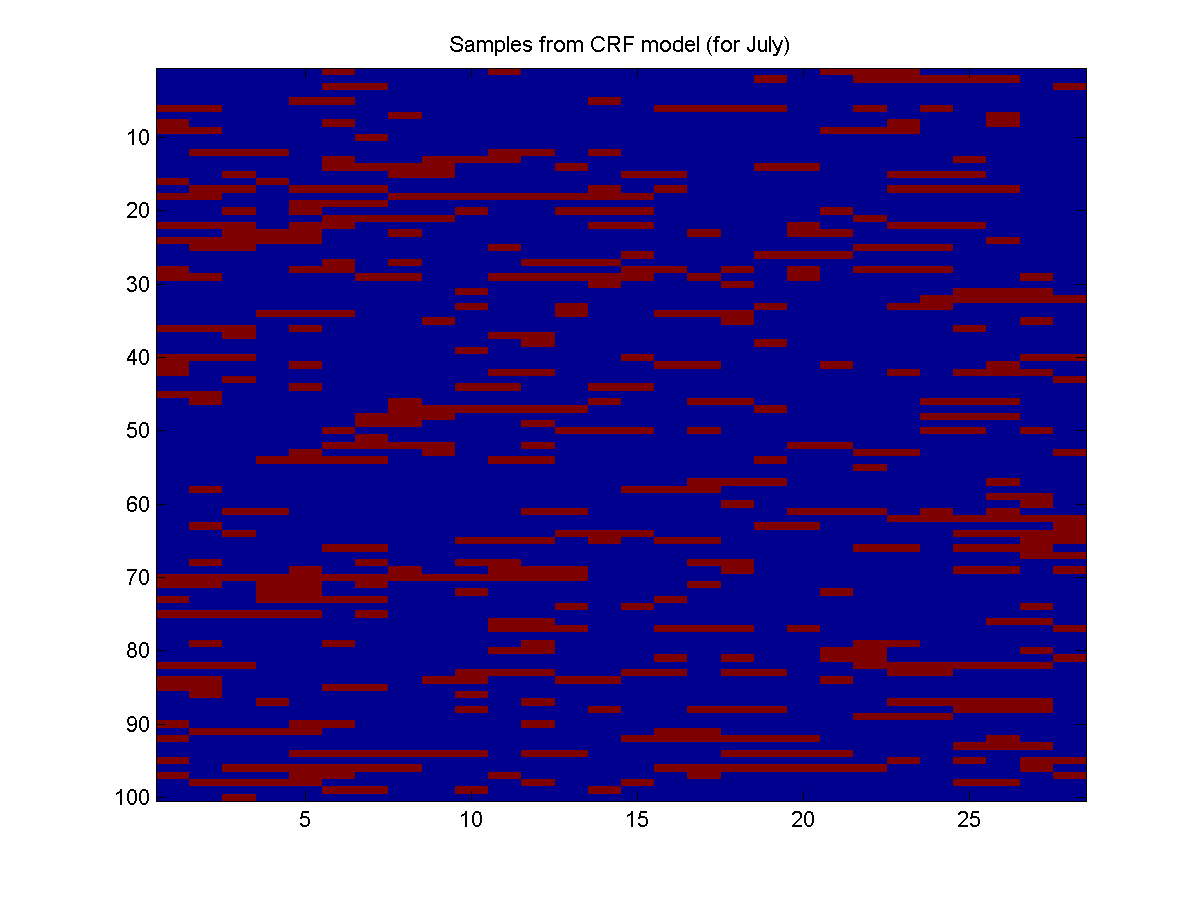
These samples seem to confirm our intuition that it rains more in December than July.

L2-Regularized Parameter Estimation

Above, we have seen that the addition of features can lead to substantially better models. However, this is still a very simple model. In practical applications of CRFs, it is not uncommon to use millions of features. In these cases, it is possible to get low values of the negative log-likelihood without having a very good model (since the negative log-likelihood decreases as we add more features to a model). This is referred to as over-fitting. One way to combat over-fitting is with L2-regularization. L2-regularization can be viewed as a penalty for having large parameter values. It is straightforward to use L2-regularization for CRFs (or MRFs) with UGM by using the penalizedL2 function. This function takes another function and values of the L2-regularization parameters, and returns the objective value (and gradient) of the function augmented with L2-regularization. Below, we give an example: % Set up regularization parameters lambda = 10*ones(size(w)); lambda(1) = 0; % Don't penalize node bias variable lambda(14:17) = 0; % Don't penalize edge bias variable regFunObj = @(w)penalizedL2(w,@UGM_CRF_NLL,lambda,Xnode,Xedge,y,nodeMap,edgeMap,edgeStruct,@UGM_Infer_Chain); % Optimize w = zeros(nParams,1); w = minFunc(regFunObj,w); NLL = UGM_CRF_NLL(w,Xnode,Xedge,y,nodeMap,edgeMap,edgeStruct,@UGM_Infer_Chain) Iteration FunEvals Step Length Function Val Opt Cond 1 2 2.99873e-05 1.90437e+04 2.55653e+03 2 3 1.00000e+00 1.76411e+04 2.33918e+03 3 4 1.00000e+00 1.72763e+04 5.65313e+02 4 5 1.00000e+00 1.72539e+04 1.94029e+02 5 6 1.00000e+00 1.72203e+04 4.66367e+02 6 7 1.00000e+00 1.71863e+04 4.26978e+02 7 8 1.00000e+00 1.71725e+04 9.30902e+01 8 9 1.00000e+00 1.71707e+04 8.04480e+01 9 10 1.00000e+00 1.71694e+04 1.34711e+02 10 11 1.00000e+00 1.71665e+04 2.03993e+02 11 12 1.00000e+00 1.71628e+04 2.00020e+02 12 13 1.00000e+00 1.71597e+04 1.81252e+02 13 14 1.00000e+00 1.71549e+04 4.18050e+01 14 15 1.00000e+00 1.71533e+04 7.63220e+01 15 16 1.00000e+00 1.71520e+04 1.35407e+02 16 17 1.00000e+00 1.71501e+04 1.57695e+02 17 18 1.00000e+00 1.71478e+04 9.84706e+01 18 19 1.00000e+00 1.71467e+04 1.40848e+01 19 20 1.00000e+00 1.71463e+04 4.76307e+01 20 21 1.00000e+00 1.71460e+04 7.27852e+01 21 22 1.00000e+00 1.71455e+04 8.87116e+01 22 23 1.00000e+00 1.71449e+04 6.67483e+01 23 24 1.00000e+00 1.71446e+04 1.75071e+01 24 25 1.00000e+00 1.71445e+04 1.77834e+01 25 26 1.00000e+00 1.71444e+04 2.74928e+01 26 27 1.00000e+00 1.71443e+04 3.80644e+01 27 28 1.00000e+00 1.71442e+04 4.73859e+01 28 29 1.00000e+00 1.71438e+04 4.55021e+01 29 30 1.00000e+00 1.71433e+04 4.03336e+01 30 32 4.93663e-01 1.71429e+04 1.96383e+01 31 33 1.00000e+00 1.71426e+04 4.42916e+00 32 34 1.00000e+00 1.71426e+04 7.80547e+00 33 35 1.00000e+00 1.71426e+04 6.56353e+00 34 36 1.00000e+00 1.71425e+04 2.32351e+00 35 37 1.00000e+00 1.71425e+04 2.84096e+00 36 38 1.00000e+00 1.71425e+04 3.88930e+00 37 39 1.00000e+00 1.71425e+04 3.93474e+00 38 40 1.00000e+00 1.71425e+04 6.13024e+00 39 42 3.79889e-01 1.71424e+04 5.21645e+00 40 43 1.00000e+00 1.71424e+04 2.93747e+00 41 44 1.00000e+00 1.71424e+04 5.06808e-01 42 45 1.00000e+00 1.71424e+04 4.22126e-01 43 46 1.00000e+00 1.71424e+04 9.28331e-01 44 47 1.00000e+00 1.71424e+04 7.80794e-01 45 48 1.00000e+00 1.71424e+04 3.99689e-01 46 49 1.00000e+00 1.71424e+04 6.24792e-01 47 50 1.00000e+00 1.71424e+04 1.40733e+00 48 51 1.00000e+00 1.71424e+04 1.81548e+00 49 52 1.00000e+00 1.71424e+04 1.19220e+00 50 53 1.00000e+00 1.71424e+04 2.22150e-01 51 54 1.00000e+00 1.71424e+04 7.59190e-02 52 55 1.00000e+00 1.71424e+04 1.00610e-01 53 56 1.00000e+00 1.71424e+04 1.16663e-01 54 57 1.00000e+00 1.71424e+04 6.81109e-02 55 59 5.02027e-01 1.71424e+04 6.86376e-02 56 60 1.00000e+00 1.71424e+04 6.01253e-02 57 61 1.00000e+00 1.71424e+04 8.71068e-02 58 62 1.00000e+00 1.71424e+04 1.11292e-01 59 63 1.00000e+00 1.71424e+04 8.80091e-02 60 65 2.88591e-01 1.71424e+04 5.69282e-02 61 66 1.00000e+00 1.71424e+04 1.04917e-02 62 67 1.00000e+00 1.71424e+04 1.08230e-02 63 68 1.00000e+00 1.71424e+04 8.98160e-03 64 69 1.00000e+00 1.71424e+04 8.42876e-03 65 70 1.00000e+00 1.71424e+04 3.26717e-03 66 71 1.00000e+00 1.71424e+04 4.21883e-03 67 72 1.00000e+00 1.71424e+04 6.02435e-03 68 73 1.00000e+00 1.71424e+04 6.57011e-03 69 74 1.00000e+00 1.71424e+04 1.47230e-02 70 75 1.00000e+00 1.71424e+04 2.70788e-03 71 76 1.00000e+00 1.71424e+04 1.49507e-03 72 77 1.00000e+00 1.71424e+04 1.12688e-03 73 78 1.00000e+00 1.71424e+04 6.33433e-04 74 79 1.00000e+00 1.71424e+04 8.52142e-04 75 80 1.00000e+00 1.71424e+04 1.62696e-03 76 81 1.00000e+00 1.71424e+04 2.34920e-03 77 82 1.00000e+00 1.71424e+04 2.19590e-03 78 83 1.00000e+00 1.71424e+04 1.36188e-03 Function Value changing by less than progTol NLL = 1.7131e+04
In the above, the optimization took fewer iterations than in the unregularized (maximum likelihood case). This is because the regularization makes the problem better-conditioned.

In the above, we follow the usual convention where the bias variables are not regularized. It is often argued that it is important to not regularize the bias variable (to avoid dependence of these weights on the scale), although in practice it often does not make a big difference if is is regularized.

As expected, the regularized estimates had a higher negative log-likelihood of the training data. However, if we carefully select the regularization parameter(s), the regularized estimates will typically have a lower negative log-likelihood than the maximum likelihood estimates on new data (ie. data that was not used for parameter estimation). Since we typically want a model that does reasonable things given new data, we will typically use a regularized estimate.

Importance of Regularization

In these demos, we will only briefly discuss regularization. However, along with choosing the right features/labels/graph, choosing the right amount of regularization will typically be crucial to the performance of the amount. Indeed, for both MRFs and CRFs the optimal parameters may not be bounded without regularization. In general, it is a good idea to use a separate regularization parameter for the edge weights than the node weights (we can accomplish this by changing the values of the lambda variable in the demo above). Then, you should perform a 2D search to find a setting of these two parameters that gives good performance on a held-out validation/test set. Without this search, CRFs often do not perform very well. In contrast, with this search then in the worst case CRFs will still perform as well as L2-regularized logistic regression (which has similar performance to support vector machines).

An alternative to L2-regularization is L1-regularization. In addition to regularizing the parameter weights, L1-regularization also encourages the weights to be exactly zero. This means that it can be used as a form of feature pruning, since features that are exactly zero can be safely removed from the model without changing anything. Using L1-regularization leads to non-differentiable optimization problems so minFunc cannot be used. But, this non-differentiable problem is highly-structured and can be solved with the related L1General package.

Notes

The main advantage of CRFs is that we don't need to build a model of the features. This is important when very complicated sets of features are needed to model the random variables, as in natural language processing and computer vision applications. CRFs are also useful when some variables are explicitly controlled in an experiment. There is no natural way to model such interventions in the random variables of undirected graphical models, but it is natural to include variables set by intervention as features in a CRF. We looked at this in:

Duvenaud Eaton Murphy Schmidt (2010). Causal learning without DAGs. Journal of Machine Learning Research Workshop and Conference Proceedings.

In this demo, the same features are used for every node and edge. You will often want to use different features for each node and edge; we will see an example of this in the next demo. However, currently UGM assumes that all nodes have the same number of features, and that all edges have the same number of features (but the number of node features doesn't have to be the same as the number of edge features). As with allowing data sets where different training examples have different graph structures, you would simply need to add up the objectives and gradients across training examples with different numbers of features in order to handle this case.

Currently, UGM only supports log-linear potentials for CRFs, but this is the most widely-used type of potential, and this parameterization is appealing since it is jointly convex in the parameters. Nevertheless, it is still possible to incorporate non-linear effects by replacing/augmenting the features with non-linear transformations of the features. Another limitation of UGM is that it does not currently support missing values or hidden variables.

CRFs were originally proposed as a model for natural language processing applications in:

Lafferty McCallum Pereira (2001). Conditional random fields: Probabilistic models for segmenting and labeling sequence data. International Conference on Machine Learning.

UGM implements a much more general notion of CRFs than described in this paper, but the cost of this generality is that several efficiencies that are available for chain-structured CRFs with high-arrity categorical features are not implemented in UGM (and further, UGM assumes that all 'sentences' have the same length). The crfChain software that I wrote with Kevin Swersky more closely resembles the type of CRF used in natural language processing: it uses an efficient storage scheme for high-arrity cateogorical features represented as indicator variables, and it naturally handles sentences of different lengths. The specific differencese between crfChain and UGM are as follows:

The 'Y' variable UGM is a nSamples by nNodes matrix, and any graph structure can be assumed of the samples. In crfChain the graph structure is forced to a chain, and the 'Y' variable is a vector that concatenates all the chains (requring a '0' in the 'position' between the chains). By always requiring the graph structure to be a chain, crfChain saves on some of the overhead required to deal with the graph structure.
In UGM, the features 'X' are assumed to be real-valued, whereas in crfChain they are assumed categorical. In UGM, you can simulate these categorical variables. If you want to simulate a categorical values that takes 's' states, simply use 's' binary indicator variables. By requiring that categorical features are used, crfChain allows a more efficient representation when the number of categories is very large.
In crfChain there are special potentials for the start and the end of the chain. This can be simuilated in UGM by adding two extra indicator features, and UGM offers even more fleixbility to do things of this nature.
In crfChain we assume a full node and edge potential parameterization and has no edge features. In contrast, UGM allows you to share parameters within the potentials, as well as have non-bias features on the edges.
In crfChain we assume that all nodes and all edges share the same parameter, whereas UGM gives you the option to allow different nodes/edges to have different parameters.

I have worked with Kevin Murphy on the Conditional Random Field Toolbox. However, UGM makes this toolbox obsolete; UGM is faster, simpler, more general, and implements more of the available methods.

PREVIOUS DEMO NEXT DEMO

Mark Schmidt > Software > UGM > TrainCRF Demo