TrainApprox UGM Demo
The last demos have considered training UGMs where exact inference is possible. However, in many cases we will not be able to do exact inference. In this demo, we consider methods for parameter estimation when exact inference is not feasible. In particular, we will consider the pseudo-likelihood approximation, as well as variational approximations. We also discuss constraining parameter estimation so that the estimated potentials are associative.
Conditional Noisy-X
In this demo we will once again consider a version of the noisy-X problem. In the conditional version of this problem, we are given pairs of images for training. In particular, for each noisy image we are also given the corresponding clean binary label. We then want to fit a conditional random field that can produce the label given the image. To make the labels y for the conditional noisy-X problem, we do the following:
load X.mat
[nRows,nCols] = size(X);
nNodes = nRows*nCols;
nStates = 2;

y = int32(1+X);
y = reshape(y,[1 1 nNodes]);
In this case, the features will correspond to a noise-corrupted version of the image:
X = X + randn(size(X))/2;
X = reshape(X,1,1,nNodes);
We now make the edgeStruct giving the lattice-structured relationship between the labels:
adj = sparse(nNodes,nNodes);

% Add Down Edges
ind = 1:nNodes;
exclude = sub2ind([nRows nCols],repmat(nRows,[1 nCols]),1:nCols); % No Down edge for last row
ind = setdiff(ind,exclude);
adj(sub2ind([nNodes nNodes],ind,ind+1)) = 1;

% Add Right Edges
ind = 1:nNodes;
exclude = sub2ind([nRows nCols],1:nRows,repmat(nCols,[1 nRows])); % No right edge for last column
ind = setdiff(ind,exclude);
adj(sub2ind([nNodes nNodes],ind,ind+nRows)) = 1;

% Add Up/Left Edges
adj = adj+adj';
edgeStruct = UGM_makeEdgeStruct(adj,nStates);
nEdges = edgeStruct.nEdges;
We now want to make the features.
Making the nodeMap and edgeMap
Given the edgeStruct and Xnode, we now consider making the nodeMap.
For the node features, we will use the intensity value at the node (as well as a bias):
% Add bias and Standardize Columns
tied = 1;
Xnode = [ones(1,1,nNodes) UGM_standardizeCols(X,tied)];
nNodeFeatures = size(Xnode,2);

nodeMap = zeros(nNodes,nStates,nNodeFeatures,'int32');
for f = 1:nNodeFeatures
    nodeMap(:,1,f) = f;
end
Unlike the previous demo, each node has different features. This is because each node will have features that depend on local properties of the image. This means that the features are different at different locations.
Note that unlike the previous demo where we only considered binary features, we now have continuous features. With continuous features, it often makes sense to do some sort of normalization of the feature values. For example, a common approach is to subtract off the mean of each feature, and normalize the values so that they have a standard deviation of 1. The function UGM_standardizeCols does this, transforming the features so that they have a mean of 0 and standard deviation of 1. Setting tied to 1 indicates that the features are to be standardized across nodes, as opposed to within nodes. Note that this standardization is optional, and in some applications it may not make sense to do it. Also, if you want to use a new data set you will need to use the same normalization used when training (and that the mean/variance of the new data may be different than the training data).
For this problem, we will use Ising-like edge potentials. For making the edge potentials, the bias should obviously be considered as a shared feature. However, the intensities of the two nodes on the edge are not a shared feature. So, we make our Xedge and edgeMap as follows:
% Make Xedge
sharedFeatures = [1 0];
Xedge = UGM_makeEdgeFeatures(Xnode,edgeStruct.edgeEnds,sharedFeatures);
nEdgeFeatures = size(Xedge,2);

% Make edgeMap
f = max(nodeMap(:));
edgeMap = zeros(nStates,nStates,nEdges,nEdgeFeatures,'int32');
for edgeFeat = 1:nEdgeFeatures
   edgeMap(1,1,:,edgeFeat) = f+edgeFeat;
   edgeMap(2,2,:,edgeFeat) = f+edgeFeat;
end
Since one of the two node features is not shared, each edge will have a total of 3 features: the bias, the intensity of the first node, and the intensity of the second.
Pseudo-likelihood Training
Performing exact inference in the conditional noisy-X model is not feasible, so we must consider approximations for parameter estimation. The first approximation we consider is known as pseudo-likelihood. The pseudo-likelihood approximation is discussed in:
- Besag (1975). Statistical analysis of non-lattice data. The Statistician.
In the pseudo-likelihood approximation, we optimize the product of conditional likelihoods instead of the joint likelihood. Because each conditional likelihood is easy to compute (the conditional UGM only has a single variable), the pseudo-likelihood approximation can be used in cases where inference is not tractable. To use UGM for pseudo-likelihood training on the conditional noisy-X problem, we can use:
nParams = max([nodeMap(:);edgeMap(:)]);
w = zeros(nParams,1);
funObj = @(w)UGM_CRF_PseudoNLL(w,Xnode,Xedge,y,nodeMap,edgeMap,edgeStruct);
w = minFunc(funObj,w);
We can analogously train an MRF with the pseudo-likelihood by making Xnode and Xedge consist of a single bias feature.
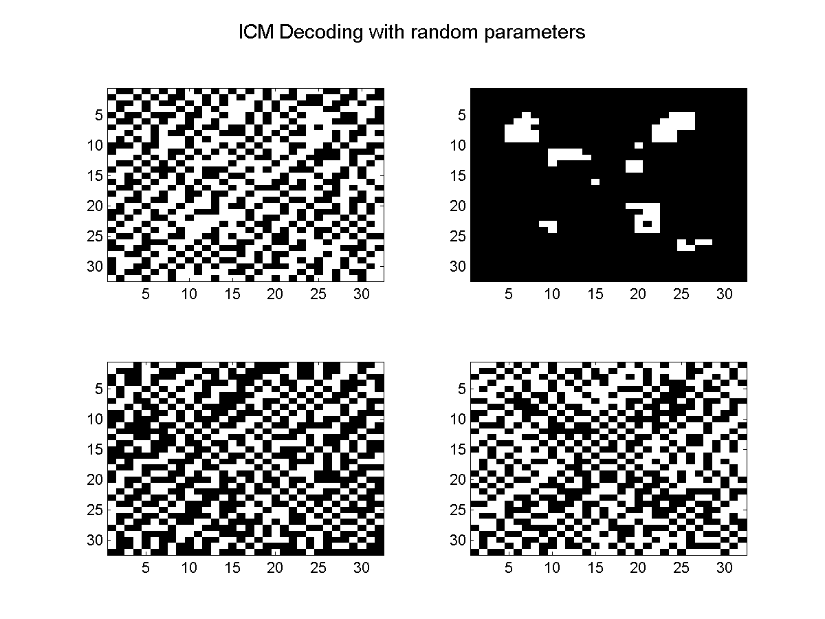
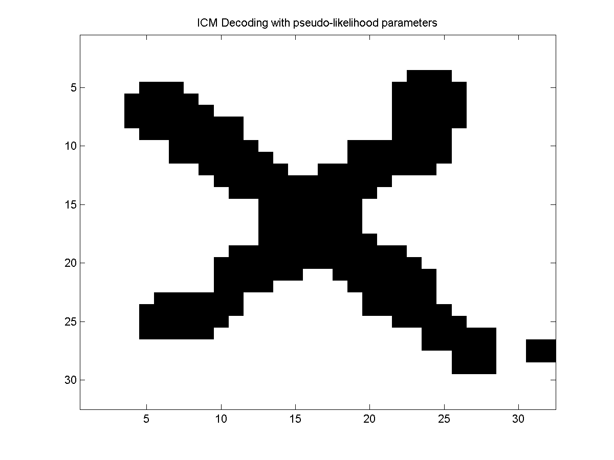
Below, we plot the results obtained using ICM decoding with random parameters, and then the results obtained using ICM decoding with the parameters estimated under the pseudo-likelihood approximation.
Associative CRFs
As discussed in the graph cuts demo, we can efficiently do exact decoding in arbitrary UGMs if the edge potentials obey an associative condition. If inference in the model is intractable but we ultimately want to use the optimal decoding(s) in the learned model, we can consider setting up the parameter estimation so that the edge potentials are guaranteed to be associative. One way to do this (for Ising-like potentials) is by enforcing that both the edge features and the edge weights are non-negative. In the case of the edge features, this is typically easy to do since we get to pick the edge features used in our model. To make the edge weights non-negative, we use a constrained optimization algorithm.
In this context we want to pick features that are likely to have an associative effect. In other words, the feature should be large if the nodes are likely to have the same value. The function UGM_makeEdgeFeaturesInvAbsDif implements one possible way to make edge features that might have an associative effect. This function assumes that shared features are non-negative, and for non-shared features it uses the reciprocal of 1 plus the absolute difference between the node features. It can be called as follows:
sharedFeatures = [1 0];
Xedge = UGM_makeEdgeFeaturesInvAbsDif(Xnode,edgeStruct.edgeEnds,sharedFeatures);
nEdgeFeatures = size(Xedge,2);
Since we have changed the edge features we must also change the edge map:
f = max(nodeMap(:));
edgeMap = zeros(nStates,nStates,nEdges,nEdgeFeatures,'int32');
for edgeFeat = 1:nEdgeFeatures
   edgeMap(1,1,:,edgeFeat) = f+edgeFeat;
   edgeMap(2,2,:,edgeFeat) = f+edgeFeat;
end
To enforce that the edge weights are non-negative, we can use a bound-constrained optimization code. In particular, to minimize the pseudo-likelihood subject to non-negativity of the edge weights, we will use minConf_TMP from the minConf package. This code requires specifying two vectors, LB and UB, containing the lower and upper bounds on the values of the variables. In our case, the node weights are unbounded and the edge weights are bounded by below from 0, so we can learn an associative CRF using the pseudo-likelihood approximation as follows:
nParams = max([nodeMap(:);edgeMap(:)]);
w = zeros(nParams,1);

funObj = @(w)UGM_CRF_PseudoNLL(w,Xnode,Xedge,y,nodeMap,edgeMap,edgeStruct); % Make objective with new Xedge/edgeMap
UB = [inf;inf;inf;inf]; % No upper bound on parameters
LB = [-inf;-inf;0;0]; % No lower bound on node parameters, edge parameters must be non-negative

w = minConf_TMP(funObj,w,LB,UB);
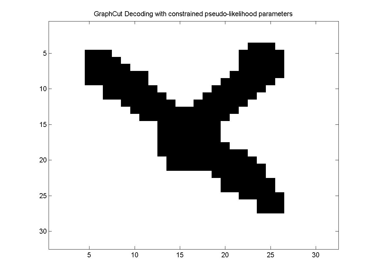
Since the estimated parameters are guaranteed to yield associative edge potentials, we can use graph cuts to find the optimal decoding in the model. Below, we plot the optimal decoding:
We proposed trainig CRFs with non-negative edge features and bound-constrained optimization so that decoding is guaranteed to be possible with graph cuts in:
- Cobzas Schmidt (2009). Increased discrimination in level set methods with embedded conditional random fields. Computer Vision and Pattern Recognition.
An interesting aspect of the constrained optimization is that it may do 'associative feature selection'. That is, it will set the edge weight to exactly 0 if the corresponding edge feature does not have an associative effect. This effectively removes the feature from the model.
Variational Inference for Training
In cases where inference is intractable, an alternative to using pseudo-likelihood is to use an approximate variational inference method. To do this with UGM, we simply replace the exact inference routine with a variational inference routine. We can train an associative CRF with loopy belief propagation for approximate inference (and the Bethe free energy approximation to the log-partition function) as follows:
w = zeros(nParams,1);
funObj = @(w)UGM_CRF_NLL(w,Xnode,Xedge,y,nodeMap,edgeMap,edgeStruct,@UGM_Infer_LBP);
w = minConf_TMP(funObj,w,LB,UB)
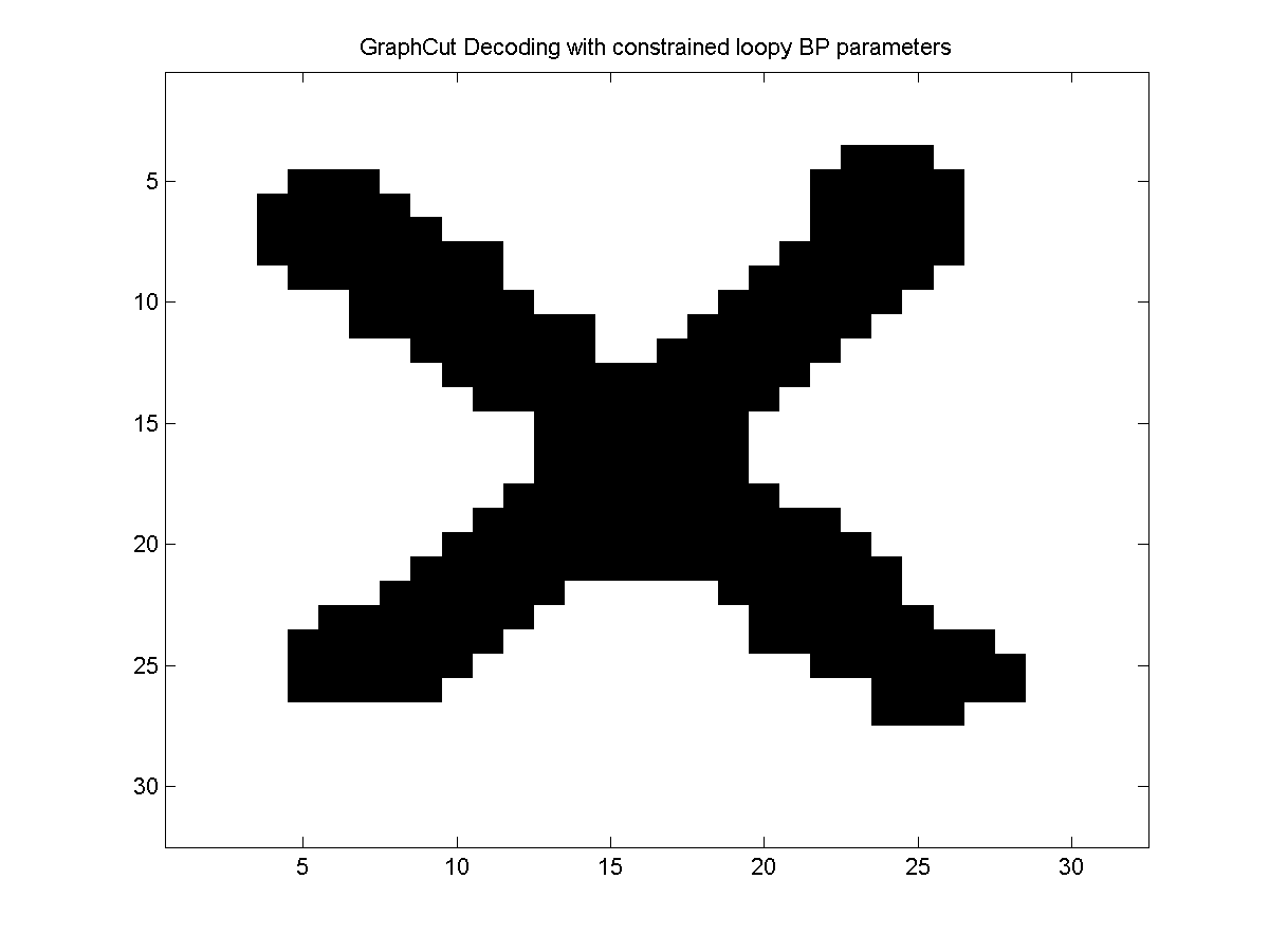
Below, we show the optimal decoding of the model trained with the loopy belief propagation approximate marginals (and approximate log-partition function):
Notes
Above, we have considered maximum likelihood and constrained maximum likelihood estimates. We could easily modify these procedures to compute regularized estimates by using the penalizedL2 function. It is also straightforward to use UGM with L1-regularization, by using one of the L1General optimization codes.
Also note that we could have replaced loopy belief propagation with a different variational inference method.
In particular, tree-reweighted belief propagation gives a convex upper bound on the negative log-likelihood function, so it leads to an optimal upper bound on the exact negative log-likelihood. In contrast, pseudo-likelihood is convex but isn't an upper bound, while loopy belief propagation isn't convex and doesn't give an upper bound.
It is also possible to enforce the associative condition with more complicated parameterizations of the edge potentials. In particular, we can enforce that the diagonal elements are positive and the non-diagonal elements are negative.
PREVIOUS DEMO NEXT DEMO
Mark Schmidt > Software > UGM > TrainApprox Demo