Suppose the graph prior is uniform over all parents sets of size <= maxFanIn. We first construct the all families log prior matrix, defined as
aflp(i,gi) = log p(parents of i = gi)which is a 5x32 matrix, since there are 2^5=32 possible parent sets. (Actually, there are only 2^4, since a node cannot include itself; the corresponding illegal entries are set to -Inf.)
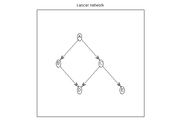
nNodes = 5;
maxFanIn = nNodes - 1;
aflp = mkAllFamilyLogPrior( nNodes, 'maxFanIn', maxFanIn );
Now let us create some data. We can sample data from the cancer network, using random CPTs, using cancerMakeData. The resulting data is stored in cancerDataObs.mat. Let us load this and compute the 5x32 all families log marginal likelihood matrix, defined as
aflml(i,gi) = sum_n log p(X(i,n) | X(gi,n))We can do this as follows:
load 'cancerDataObs.mat' % from cancerMakeData
% data is size d*N (nodes * cases), values are {1,2}
aflml = mkAllFamilyLogMargLik( data, 'nodeArity', repmat(2,1,nNodes), ...
			       'impossibleFamilyMask', aflp~=-Inf, ...
			       'priorESS', 1);
This uses ADtrees to cache the sufficient statistics (see Moore98 for
details). This is implemented in C.
If we have Gaussian data, we can use the BGe score instead:
aflml = mkAllFamilyLogMargLik( data, 'impossibleFamilyMask', aflp~=-Inf,
  'cpdType', 'gaussian' );
Finally we are ready to compute the optimal DAG
optimalDAG = computeOptimalDag(aflml); % MLE, max p(D|G)
%optimalDAG = computeOptimalDag(aflml+aflp); % MAP, max p(D,G)
We can also compute exact edge marginals using DP:
epDP = computeAllEdgeProb( aflp, aflml );In this simple setting, we can compute exact edge marginals by brute force enumeration over all 29,281 DAGs of 5 nodes:
epEnumer = computeAllEdgeProb_Exact(0, aflml); % 0 denotes uniform priorIf we visualize these heat maps, we see that they are different. (DP in top left is not the same as enumeration in bottom right.) This is because the DP algorithm implicitly assumes a special "modular" prior; see Friedman03 and Koivisto04. We will fix this below using MCMC sampling.
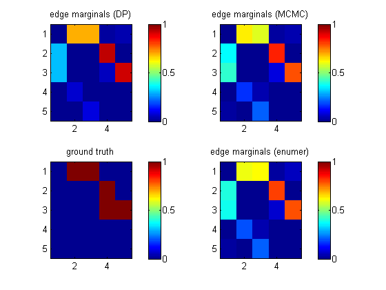
[samples, diagnostics, runningSum] = sampleDags(@uniformGraphLogPrior, aflml, ...
				    'burnin', 100, 'verbose', true, ...
				    'edgeMarginals', epDP, 'globalFrac', 0.1, ...
				    'thinning', 2, 'nSamples', 5000);
epMCMC = samplesToEdgeMarginals(samples);
The heat map above (top right) shows that this gives the same results as exhaustive enumeration with a uniform prior. The MCMC routine uses hash tables to represent samples of graphs compactly.
Order sampling (Friedman03) is in the OrderMcmc directory, but is undocumented. We also support the importance sampling reweighting of Ellis06.
Let us load some data where we have performed a perfect intervention on node A. The 5x700 matrix clamped is defined so clamped(i,n)=1 iff node i is set by intervention in case n. We modify the computation of the marginal likelihoods to remove cases that were set by intervention.
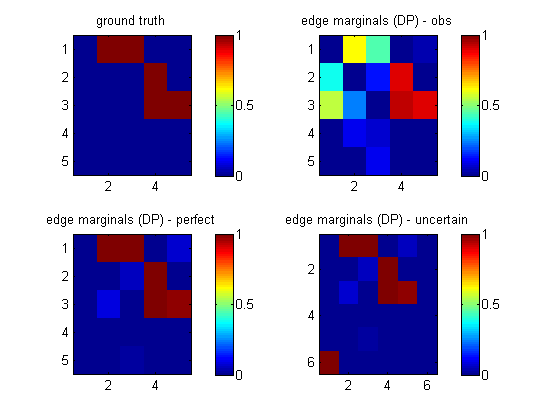
load 'cancerDataInterA.mat' % from cancerMakeData
nNodes = 5;
maxFanIn = nNodes - 1;
aflp = mkAllFamilyLogPrior( nNodes, 'maxFanIn', maxFanIn );
aflml_perfect = mkAllFamilyLogMargLik( data, 'nodeArity', repmat(2,1,nNodes), ...
			       'impossibleFamilyMask', aflp~=-Inf, ...
			       'priorESS', 1, ...
			       'clampedMask', clamped);
epDP_perfect = computeAllEdgeProb( aflp, aflml_perfect );
This lets us recover the true structure uniquely. If we ignore the fact that this is interventional data (by omitting the clamped parameter), we get the wrong answer, as shown in the top right plot below (labeled 'obs').
Let us call the intervention node number 6. This node is always clamped; let us put it in state 1 half the time, and state 2 for the rest, and append this to the normal data.
N = size(data,2);
nObservationCases = N/2; % # observational data cases
nInterventionCases = N/2; % no interventions
assert(N==nObservationCases+nInterventionCases);
data_uncertain = [data; [ones(1,nObservationCases) 2*ones(1,nInterventionCases)]];
clamped_uncertain = [zeros(size(clamped)); ones(1,N)];
When learning the topology, we do not want to allow connections between the intervention nodes, or back from the backbone nodes to the intervention nodes. We can enforce this by putting the intevention node in layer 1, and the other nodes in layer 2, and restricting the fan-in between and within layers as follows
% fan-in
%     L1  L2
% L1   0   1    % only 1 intervention parent allowed for L2 nodes
% L2   0   max  % only max # paretns allowed in total for L2 nodes

maxFanIn_uncertain = [ 0 1 ; 0 maxFanIn ];
layering = [2*ones(1,nNodes) 1];
nodeArity = 2*ones(1,nNodes);
nodeArity_uncertain = [nodeArity 2];

aflp_uncertain = mkAllFamilyLogPrior( nNodes+1, 'maxFanIn', maxFanIn_uncertain, ...
				      'nodeLayering', layering );

aflml_uncertain = mkAllFamilyLogMargLik(data_uncertain, ...
		'nodeArity', nodeArity_uncertain, 'clampedMask', clamped_uncertain, ...
		'impossibleFamilyMask', aflp_uncertain~=-Inf, 'verbose', 0 );

epDP_uncertain = computeAllEdgeProb( aflp_uncertain, aflml_uncertain );
We see from the picture above (bototm right, labeled 'uncertain') that we learn that node 6 targets node 1 (A), and we also correctly recover the backbone.
For example, suppose nodes (1,3) are in layer 1 and nodes (2,4,5) are in layer 2. We can allow connections from L1 to L2, and within L2, as follows:
layering = [1 2 1 2 2 ];
maxFanIn = [0 -1 ; 0 3 ];
M(1,1)=0 means no connections into L1. M(1,2)=-1 means no constraints on the number of L1->L2 connections (modulo constraints imposed by M(2,2)); M(2,2)=3 means at most 3 parents for any node in L2.
myDrawGraph(dag, 'labels', labels, 'layout', graphicalLayout)If the layout coordinates are omitted, the function lays the nodes out in a circle.
To achieve higher quality results, I recommend the free windows program called pajek. A function adj2pajek2.m will convert a dag to the pajek format; this file can then be read in and automatically layed out in a pretty way.
 |
 |
@inproceedings{Eaton07_jmlr,
  author = "D. Eaton and K. Murphy",
 title = {{Belief net structure learning  from uncertain interventions}},
 journal = jmlr,
 note= "Submitted",
 year = 2007,
 url = "http://www.cs.ubc.ca/~murphyk/Papers/jmlr07.pdf"
}

@inproceedings{Eaton07_aistats,
  author = "D. Eaton and K. Murphy",
 title = {{Exact Bayesian structure learning from uncertain interventions}},
 booktitle = "AI/Statistics",
 year = 2007
 url = "http://www.cs.ubc.ca/~murphyk/Papers/aistats07.pdf"
}

@inproceedings{Eaton07_uai,
  author = "D. Eaton and K. Murphy",
 title = {{Bayesian structure learning using dynamic programming and MCMC}},
 booktitle = uai,
 year = 2007,
 url = "http://www.cs.ubc.ca/~murphyk/Papers/eaton-uai07.pdf"
}

@inproceedings{Ellis06,
 title = {{Sampling Bayesian Networks quickly}},
 author = "B. Ellis and W. Wong",
 booktitle = "Interface",
 year = 2006
}

@article{Friedman03,
 title = {{Being Bayesian about Network Structure: A Bayesian Approach to Structure Discovery in Bayesian Networks}},
 author = "N. Friedman and D. Koller",
  journal = "Machine Learning",
 volume = 50,
  pages = "95-126",
 year = 2003
}

@article{Husmeier03,
 author = "D. Husmeier",
 title = {{Sensitivity and specificity of inferring genetic regulatory
interactions from microarray experiments with dynamic Bayesian networks}},
 journal = "Bioinformatics",
 volume = 19,
 pages = "2271--2282",
 year = 2003
}

@article{Koivisto04,
 author = "M. Koivisto and K. Sood",
 title = {{Exact Bayesian structure discovery in Bayesian networks}},
 journal = jmlr,
 year = 2004,
 volume = 5,
 pages = "549--573",
url = {{http://www.ai.mit.edu/projects/jmlr//papers/volume5/koivisto04a/koivisto04a.pdf}}}

@inproceedings{Koivisto06,
 author = "M. Koivisto",
 title = {{Advances in exact Bayesian structure discovery in Bayesian networks}},
 booktitle = uai,
 year = 2006,
 url = {http://www.cs.helsinki.fi/u/mkhkoivi/publications/uai-2006.pdf}
}

@article{Moore98,
    author = "A.  Moore and M. Lee",
    title = "Cached Sufficient Statistics for Efficient Machine Learning with Large Datasets",
    journal = jair,
    volume = "8",
    pages = "67-91",
    year = "1998"
   url = "citeseer.nj.nec.com/moore97cached.html"
}


@inproceedings{Ott04,
 title = "Finding optimal models for small gene networks",
 author = "Sascha Ott and Seiya Imoto and Satoru Miyano",
 booktitle= "Pacific Symposium on Biocomputing",
 year = 2004
 url = "http://helix-web.stanford.edu/psb04/ott.pdf"
}


@article{Sachs05,
 title = "Causal Protein-Signaling Networks Derived from Multiparameter Single-Cell Data",
 author = "K. Sachs and O. Perez and D. Pe'er and D. Lauffenburger and G. Nolan",
 journal = "Science",
 year = 2005,
  volume = 308,
 page = "523"
}

@inproceedings{Silander06,
 author = "T. Silander and P. Myllymaki",
  title = {{A simple approach for finding the globally optimal Bayesian network structure}},
  year = 2006,
  booktitle = uai,
  url = {{http://eprints.pascal-network.org/archive/00002135/01/main.pdf}}
}

@article{Werhli07,
 author = "A. Werhli and D. Husmeier",
 title = "Reconstructing Gene Regulatory Networks with Bayesian
Networks by Combining Expression Data with Multiple Sources of Prior Knowledge",
 journal = "Statistical Applications in Genetics and Molecular Biology",
 year = 2007,
 volume = 6,
 number = 1
}