Contents

Set-up repeatable randomness for demo

seed = 0;
rand('seed', seed);
randn('seed', seed);

Create a Bayes net based on the 'Cancer' topology

labels = {'A','B','C','D','E'};

dag = zeros(5);
A = 1; B = 2; C = 3; D = 4; E = 5;
dag(A,[B C]) = 1;
dag(B,D) = 1;
dag(C,[D E]) = 1;

sz = 2*ones(5,1);
bnet =  mk_bnet(dag, sz);

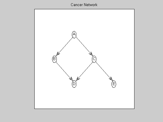
Visualize the ground-truth graph

graphicalLayout = [0.4000 0.2000 0.6000 0.4000 0.8000 ; ...
	0.7500 0.5000 0.5000 0.2500 0.2500 ]; % in normalized [0..1]x[0..1] Matlab plotting coordinates
figure;
myDrawGraph(dag, 'labels', labels, 'layout', graphicalLayout);
title('Cancer Network');

Generate a tabular CPD (multinomial model) on each node

p = .9;
cptA = [.4 .6];
cptB = [1-p p ; p 1-p];
cptC = [1-p p ; p 1-p];
cptD = zeros(2, 2, 2);
cptD(:,:,1) = [ .15 .3 ; .7 .9];
cptD(:,:,2) = 1-cptD(:,:,1);
cptE = [p 1-p ; 1-p p];

bnet.CPD{A} = tabular_CPD(bnet, A, 'CPT', cptA);
bnet.CPD{B} = tabular_CPD(bnet, B, 'CPT', cptB);
bnet.CPD{C} = tabular_CPD(bnet, C, 'CPT', cptC);
bnet.CPD{D} = tabular_CPD(bnet, D, 'CPT', cptD);
bnet.CPD{E} = tabular_CPD(bnet, E, 'CPT', cptE);

nNodes = length(dag);

Generate data from the Bayes net

nObservationCases = 350; % # observational data cases
nInterventionCases = 0; % no interventions
interventions = {};
[data clamped] = mkData(bnet, nObservationCases, interventions, nInterventionCases );

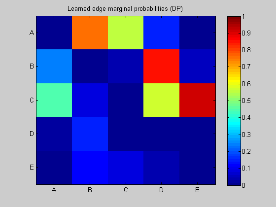
Use DP algorithm to re-learn the structure

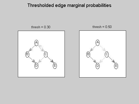
maxFanIn = nNodes - 1; % do not restrict the fan-in of any node

aflp = mkAllFamilyLogPrior( nNodes, 'maxFanIn', maxFanIn ); % construct the modular prior on all possible local families
aflml = mkAllFamilyLogMargLik( data, 'nodeArity', repmat(2,1,nNodes), 'impossibleFamilyMask', aflp~=-Inf); % compute marginal likelihood on all possible local families
ep = computeAllEdgeProb( aflp, aflml ); % compute the marginal edge probabilities using

figure;
imagesc(ep, [0 1 ]);
title('Learned edge marginal probabilities (DP)');
set(gca, 'XTick', 1:5);
set(gca, 'YTick', 1:5);
set(gca, 'XTickLabel', labels);
set(gca, 'YTickLabel', labels);
colorbar;

figure;
subplot(1,2,1);
thresh = 0.3;
myDrawGraph(ep, 'labels', labels, 'layout', graphicalLayout, 'thresh', thresh);
title(sprintf('thresh = %0.2f', thresh));

subplot(1,2,2);
thresh = 0.5;
myDrawGraph(ep, 'labels', labels, 'layout', graphicalLayout, 'thresh', thresh);
title(sprintf('thresh = %0.2f', thresh));

suptitle('Thresholded edge marginal probabilities');

fprintf('Simulation paused. Press any key to continue.');
pause

Simulation paused. Press any key to continue.

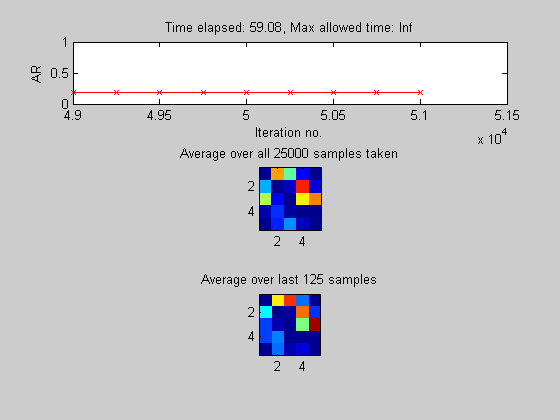
Use MCMC (Hybrid, Local/Global mixture proposal) to correct the bias induced by modular prior

use a uniform prior on structures

[samples, diagnostics] = sampleDags(@uniformGraphLogPrior, aflml, 'burnin', 1000, 'verbose', true, ...
    'edgeMarginals', ep, 'koivistoFrac', .1, 'thinning', 2, 'nSamples', 25000);
epMcmc = samplesToEdgeMarginals(samples); % average the DAG samples to empirically estimate the edge marginals

Sample 1000 of 51000 [ar=0.198]
Sample 2000 of 51000 [ar=0.194]
Sample 3000 of 51000 [ar=0.180]
Sample 4000 of 51000 [ar=0.191]
Sample 5000 of 51000 [ar=0.194]
Sample 6000 of 51000 [ar=0.191]
Sample 7000 of 51000 [ar=0.188]
Sample 8000 of 51000 [ar=0.186]
Sample 9000 of 51000 [ar=0.185]
Sample 10000 of 51000 [ar=0.186]
Sample 11000 of 51000 [ar=0.184]
Sample 12000 of 51000 [ar=0.184]
Sample 13000 of 51000 [ar=0.184]
Sample 14000 of 51000 [ar=0.184]
Sample 15000 of 51000 [ar=0.184]
Sample 16000 of 51000 [ar=0.184]
Sample 17000 of 51000 [ar=0.183]
Sample 18000 of 51000 [ar=0.182]
Sample 19000 of 51000 [ar=0.182]
Sample 20000 of 51000 [ar=0.181]
Sample 21000 of 51000 [ar=0.182]
Sample 22000 of 51000 [ar=0.182]
Sample 23000 of 51000 [ar=0.182]
Sample 24000 of 51000 [ar=0.182]
Sample 25000 of 51000 [ar=0.180]
Sample 26000 of 51000 [ar=0.180]
Sample 27000 of 51000 [ar=0.180]
Sample 28000 of 51000 [ar=0.181]
Sample 29000 of 51000 [ar=0.181]
Sample 30000 of 51000 [ar=0.179]
Sample 31000 of 51000 [ar=0.179]
Sample 32000 of 51000 [ar=0.180]
Sample 33000 of 51000 [ar=0.180]
Sample 34000 of 51000 [ar=0.181]
Sample 35000 of 51000 [ar=0.181]
Sample 36000 of 51000 [ar=0.181]
Sample 37000 of 51000 [ar=0.182]
Sample 38000 of 51000 [ar=0.182]
Sample 39000 of 51000 [ar=0.182]
Sample 40000 of 51000 [ar=0.182]
Sample 41000 of 51000 [ar=0.182]
Sample 42000 of 51000 [ar=0.182]
Sample 43000 of 51000 [ar=0.182]
Sample 44000 of 51000 [ar=0.182]
Sample 45000 of 51000 [ar=0.182]
Sample 46000 of 51000 [ar=0.182]
Sample 47000 of 51000 [ar=0.181]
Sample 48000 of 51000 [ar=0.180]
Sample 49000 of 51000 [ar=0.181]
Sample 50000 of 51000 [ar=0.181]
Sample 51000 of 51000 [ar=0.182]

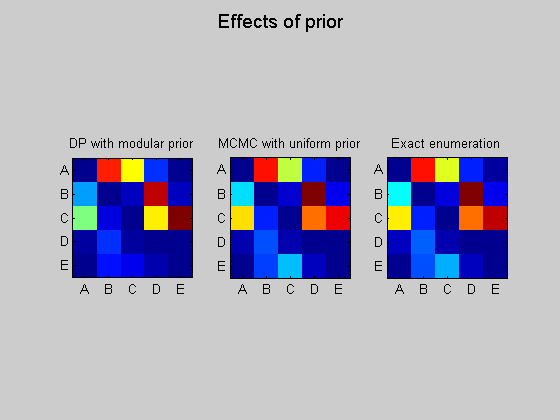
Use exhaustive enumeration (sum over super-exponential space of DAGs) to compute exact answer (for a uniform prior)

(DP algorithm is exact too, but only for the restricted "modular" prior)

epExact = computeAllEdgeProb_Exact(0, aflml); % 0 denotes uniform prior

figure;
subplot(1,3,1);
imagesc(ep);
set(gca, 'XTick', 1:5);
set(gca, 'YTick', 1:5);
set(gca, 'XTickLabel', labels);
set(gca, 'YTickLabel', labels);
title('DP with modular prior');
axis('square');

subplot(1,3,2);
imagesc(epMcmc);
set(gca, 'XTick', 1:5);
set(gca, 'YTick', 1:5);
set(gca, 'XTickLabel', labels);
set(gca, 'YTickLabel', labels);
title('MCMC with uniform prior');
axis('square');

subplot(1,3,3);
imagesc(epExact);
set(gca, 'XTick', 1:5);
set(gca, 'YTick', 1:5);
set(gca, 'XTickLabel', labels);
set(gca, 'YTickLabel', labels);
title('Exact enumeration');
axis('square');

suptitle('Effects of prior');

loading Cache/DAGS5.mat
likelihood 10000/29281
likelihood 20000/29281
marginals 10000/29281
marginals 20000/29281

Published with MATLAB® 7.3