ICM UGM Demo
The last demo ends the first series of demos coverings exact methods for
decoding/inference/sampling. We now turn to the case of approximate
methods. These methods can be applied to models with general graph
structures and edge potentials, but don't necessarily perform these
operations exactly. This first demo discusses approximate decoding with
local search, generalizing the iterated conditional mode (ICM) algorithm mentioned in the previous demo.
Iterated Conditional Modes
The ICM algorithm is one of the simplest methods for optimal decoding. In the
ICM algorithm, we initialize the nodes to some starting state values (by default, UGM uses
the states that maximize the node potentials), and we then start cycling through the nodes in order. When we get to
node i, we consider all states that node i could take, and
replace its current state with the state that maximizes the joint potential.
We keep cycling through the nodes in order until we complete a full cycle
without changing any nodes.
At this point, we have reached a local optima of the joint potential that can not be improved by changing the state of any single node.
The ICM algorithm is described in Besag's paper on analyzing
"dirty pictures":
- J.E. Besag. On the Statistical Analysis of Dirty Pictures. Journal of
the Royal Statistical Society Series B, 1986.
In UGM, we can apply ICM using:
getNoisyX
ICMDecoding = UGM_Decode_ICM(nodePot,edgePot,edgeStruct);
figure;
imagesc(reshape(ICMDecoding,nRows,nCols));
colormap gray
This function UGM_Decode_ICM can also take an optional fourth argument that gives the intial configuration.
Greedy Local Search Decoding
The ICM algorithm is a specific instance of a local search discrete
optimization algorithm, sometimes described as a first improvement
greedy algorithm. Instead of this particular local search method, we could
instead consider other local search methods.
As one example, we could consider a best improvement greedy algorithm,
where we search for the single state change that improves the joint
potential by the largest amount. This is slightly more expensive than ICM
since we only make a single state change after cycling through the nodes, but
it ensures that we always take the 'best'
move at each iteration.
In UGM we can apply this greedy algorithm using:
greedyDecoding = UGM_Decode_Greedy(nodePot,edgePot,edgeStruct);
figure;
imagesc(reshape(greedyDecoding,nRows,nCols));
colormap gray
This function can also take an optional fourth argument that gives the initial configuration.
ICM with Restarts
A much more effective enhancement of the ICM algorithm is to restart it (with a
different initial configuration) whenever it reaches a local optima. By doing
this, we may be able to explore different local optima. Further, if we restart
it enough times (and guarantee that our restart mechanism eventually generates
all configurations), this procedure will eventually find the global optima.
In UGM we can run the ICM algorithm with 1000 restarts using:
nRestarts = 1000;
ICMrestartDecoding = UGM_Decode_ICMrestart(nodePot,edgePot,edgeStruct,nRestarts);
figure;
imagesc(reshape(ICMrestartDecoding,nRows,nCols));
colormap gray
Comparison
Applying the the three methods to a sample of the noisy X problem yields the
following results:
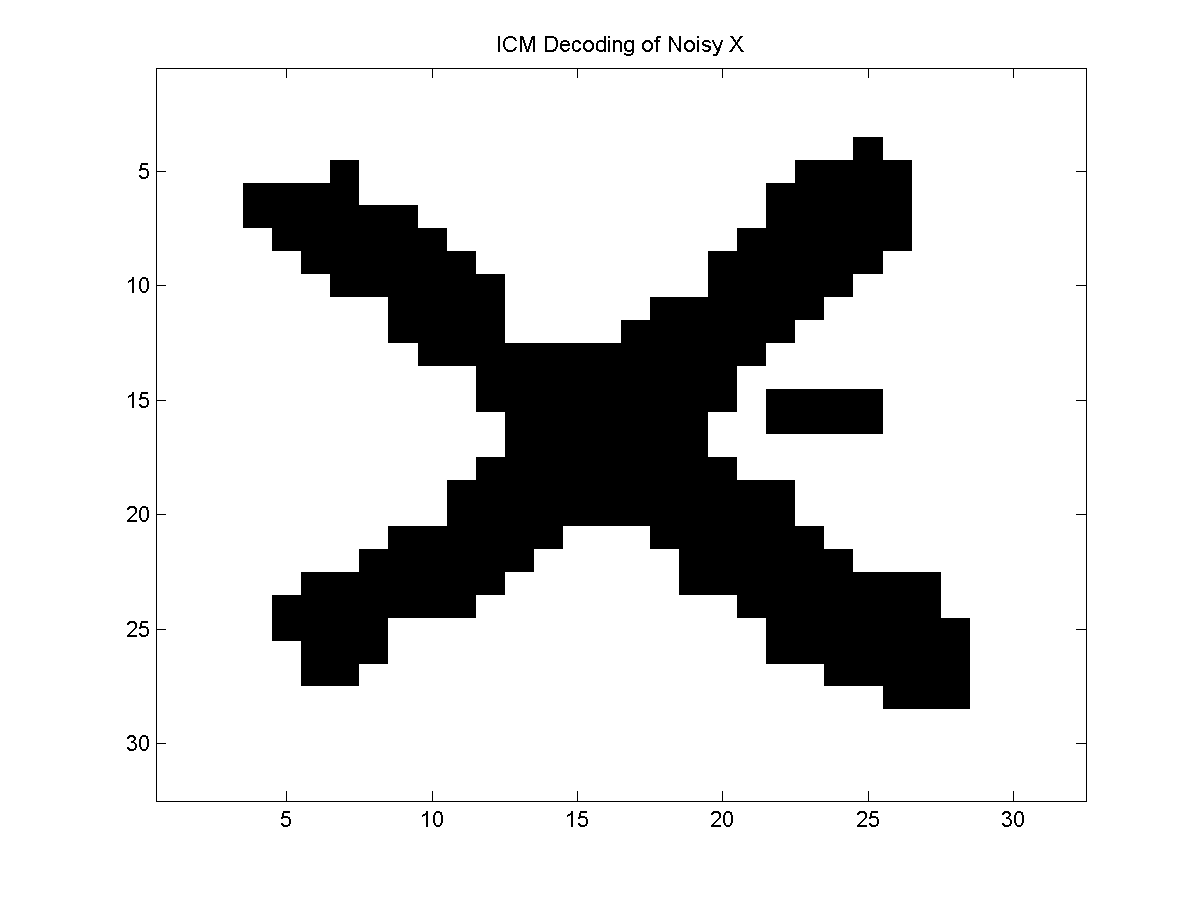
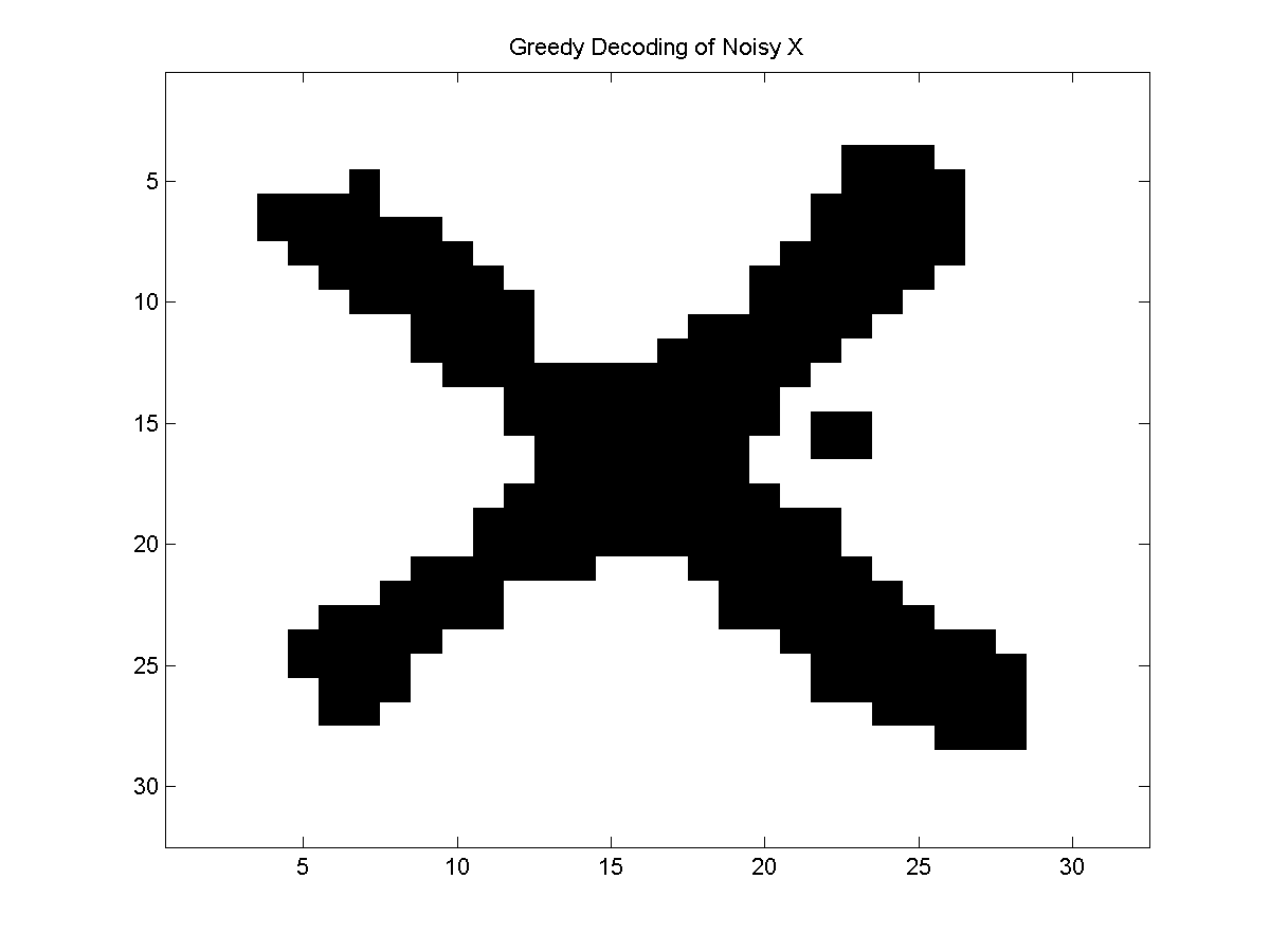
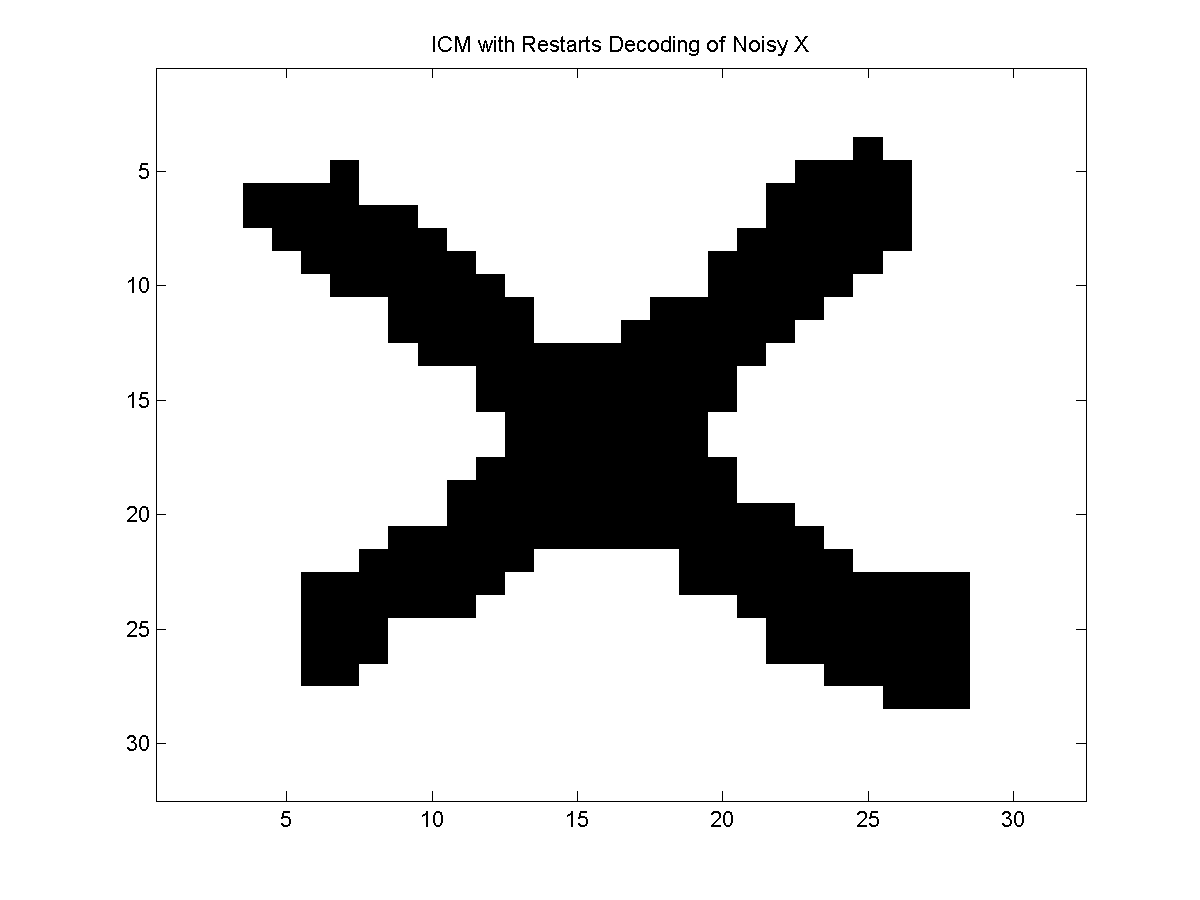
In this example, the best-improvement greedy decoding did slightly better than
the ICM algorithm, but the (stochastic) ICM with restarts algorithm did better
than both of the deterministic strategies.
Notes
These are just three of the many possible local search methods that could be
applied.
For example, you could use any of the
algorithms from the inside cover of "Stochastic Local Search: Foundations and Applications" by Hoos and Stutzle.
This includes things like local search methods with stochastic moves, dynamic local search methods, iterated local search
methods, genetic algorithms, ant colony optimization, etc.
PREVIOUS DEMO NEXT DEMO
Mark Schmidt > Software > UGM > ICM Demo