Matlab Software from "Graphical Model Structure Learning with L1-Regularization"
By Mark
Schmidt (2010)
Last updated 3 February 2012.
Summary
This package contains the code used to produce the results in my thesis:
Roughly, there are five components corresponding to five of the thesis chapters:
- Chapter 2: L-BFGS methods for optimizing differentiable functions plus an L1-regularization term.
- Chapter 3: L-BFGS methods for optimizing differentiable functions with simple constraints or regularizers.
- Chapter 4: An L1-regularization method for learning dependency networks, and methods for structure learning in directed acyclic graphical models.
- Chapter 5: L1-regularization and group L1-regularization for learning undirected graphical models, using either the L2, Linf, or nuclear norm of the groups.
- Chapter 6: Overlapping group L1-regularization for learning hierarhical log-linear models, and an active set method for searching through the space of higher-order groups.
Clicking on the image below opens the slides used during my defense, which
briefly overview the methods and some results:
Clicking on the image below opens the slides of a longer talk that covers some
of the material from Chapters 2-3:
Clicking on the image below opens the slides of another talk that
covers some of the material from Chapters 5-6.
Below are more detailed overviews of the five packages.
Chapter 2: L1General
This package contains a variant on the L1General code that implements a variety of solvers for optimization with L1-regularization. Specifically, they solve the problem:
min_w: funObj(w) + sum_i lambda_i|w_i|,
where funObj(w) is a differentiable function of the parameter vector w and lambda is a vector of non-negative hyper-parameter specifying the scale of the penalty on each element in w.
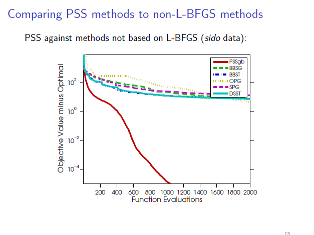
While the previous L1General code focused on methods that require explicit Hessian calcluation or storing a dense Hessian approximation, this variant ('L1General2') concentrates on limited-memory solvers that can solve problems with millions of variables. Specifically, the following methods are available (see Chapter 2 for details):
- L1General2_SPG: Spectral projected gradient.
- L1General2_BBST: Barzilai-Borwein soft-threshold.
- L1General2_BBSG: Barzilai-Borwein sub-gradient.
- L1General2_OPG: Optimal projected gradient.
- L1General2_DSST: Diagonally-scaled soft-threshold.
- L1General2_OWL: Orthant-wise learning.
- L1General2_AS: Active set.
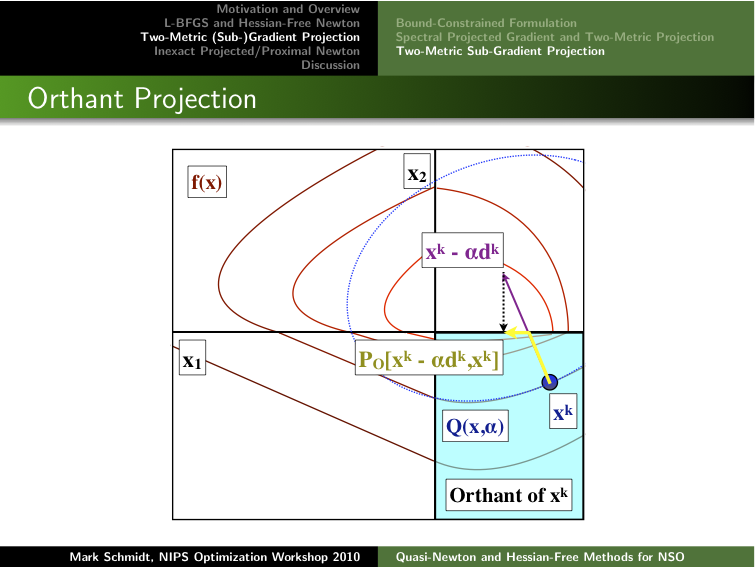
- L1General2_TMP: Two-metric projection.
- L1General2_PSSgb: Projected scaled sub-gradient (Gafni-Bertsekas variant).
- L1General2_PSSsp: Projected scaled sub-gradient (sign projection variant).
- L1General2_PSSas: Projected scaled sub-gradient (active set variant).
In subsequent work, the PSS methods are sometimes referred to as 'two-metric sub-gradient projection' methods.
Usage
The methods have a simple common interface. As an example, to call the L1General_PSSgb method you can use:
>> w = L1General_PSSgb(funObj,w,lambda,options);
The input parameters are:
- funObj: a function handle for a function
that treutnrs the objective and gradient value for a given parameter vector.
- x0: the initial guess to the optimal
solution (this could simply be the zero vector of appropriate size).
- v: a vector giving the regularization
weights, where each element must be greater than or equal to zero.
- options: a structure whose fields specify
parameters of the optimization. To use the default options, simply
set options = [] or omit the last argument.
The possible fields to set in the options structure are:
- options.corrections: the number of corrections to store for the
methods based on L-BFGS. The default value is 100, which is reasonable when
optimizing graphical models but may be high in other applications (where a
more appropriate value might be 5 or 10).
- options.optTol: The method will exit if the optimality tolerance is
below this threshold.
- options.progTol: The method will exist if the amount of progress is
below this threshold.
- options.maxIter: The method will exit if it exceeds this number of
evaluations of funObj.
- options.quadraticInit: Set this to 1 to use a quadratic
initialization of hte line search. This can achieve better performance
for problems where backtracking steps are required on each iteration.
- options.verbose: If you are confident the method will find the
correct solution, set this to 0 for best performance.
Examples
The function demo_L1General shows how to use the various solvers to find the solution of an L1-regularized logistic regression problem.
The function demo_L1Generalpath shows how to use one of the solvers for computing the optimal solution for several values of lambda, by
using the solution for one value of lambda as the initial guess to the solution
for the next value. The function demo_L1Generalpath
also demonstrates how an active set strategy (described in Section 2.5) can be used to substantially reduce the computational costs for values of
lambda where the solution is very sparse.
A variety of other examples of L1-regularization problems that can be solved with L1General
can be
found on
the examples
of using L1General page,
including: LASSO, elastic net, probit regression,
smooth support vector machines, multinomial logistic regression, non-parametric logistic
regression, graphical LASSO, neural networks, Markov random fields, conditional
random fields.
Chapter 3: minConf
This is an update to the minConf package. Like previous versions, it contains solvers for the problem of minimizing a different function over a 'simple' closed convex set:
min_w: funObj(w), subject to w is in C.
However, this new version also includes analogous methods for unconstrained optimization of the sum of a differentiable function and a 'simple' convex function:
min_w: funObj(w) + regObj(w).
Unlike funObj, the function regObj does not need to be differentiable. Though it does not necessarily have to be a regularization function, we refer to regObj as the 'regularizer'. In this update of minConf, the following methods are available (see Chapter 3 for details):
- minConf_SPG: Spectral projected gradient method for optimization over simple convex sets.
- minConf_OPG: Optimal projected gradient method for optimization over simple convex sets.
- minConf_PQN: Projected quasi-Newton method for optimization over simple convex sets.
- minConf_BBST: Barzilai-Borwein soft-threshold method for optimization with simple regularizers.
- minConf_QNST: Quasi-Newton soft-threshold method for optimization with simple regularizers.
Usage
The methods have a simple common interface. As an example, to call the minConf_SPG method you can use:
>> w = minConf_SPG(funObj,w,funProj,options);
The third argument is a function handle for a function that computes the projection on to the convex set. That is,
funProj(w) = argmin_x: (1/2)||x-w||^2, s.t. x is in C.
In the case of the 'soft-threshold' methods for optimizing with a simple
regularizer, funProj is a function handle that returns the solution of the proximal problem:
funProj(w,t) = argmin_x: (1/2)||x-w||^2 + t*r(x).
Details on the available options are available from the minConf webpage.
Group L1-Regularization
In Chapter 3, these optimization methods were discussed in the context of optimizing a differentiable function with group L1-regularization:
min_w: funObj(w) + sum_g lambda_g ||w_g||_2,
Here, each group 'g' is a set of parameters that we want to encourage to be jointly sparse. The function L1GeneralGroup_Auxiliary and L1GeneralGroup_SoftThresh use the minConf functions to solve problems of this form. They have the interface:
>> w = L1GeneralGroup_Auxiliary(funObj,w,lambda,groups,options);
The lambda variable specifies the degree of regularization for each
group; the length of lambda must be equal to the number of groups.
The groups variable is a vector that is the same length as w,
where each element specifies which group the corresponding variable belongs to.
These assignements can be from 1 up to the number groups (the length
of lambda), or they can be set to zero if the corresponding variable is
not regularized. In addition to specifying options of the optimization
procedure, these two functions also have two extra options:
options.method allows you to select the optimization method that will be
used, and options.norm allows you to penalize different norms of the
groups.
Examples
The function demo_minConf shows how to use the various solvers to find the solution of a group L1-regularized multi-task logistic regression problem.
The function demo_minConfpath shows how to use one of the solvers for computing the optimal solution for several values of lambda, by
using the solution for one value of lambda as the initial guess to the solution for the next value.
The function demo_minConfpath
also demonstrates how an active set strategy (described in Section 3.4) can be used to substantially reduce the computational costs for values of
lambda where the solution is very sparse. This demo first computes the regularization path when penalizing the sum of the L2-norms of the groups, and subsequently computes the regularization path when penalizing the Linf-norms of the groups.
A variety of other examples of problems that can be solved with minConf_PQN can be
found on the examples
of using PQN page,
including:
problems with simplex constraints or (complex) L1-ball constraints,
group-sparse regression with categorical features, group-sparse multi-task
regression/classification, group-sparse multionomial classification,
blockwise-sparse Gaussian graphical models, regularization with the
'over-LASSO', kernelzed support vector machines and multiple kernel learning in
the primal, approximating node marginals in graphical models with the mean field
approximation, structure learning in multi-state Markov random fields and
conditional random fields.
A variety of the regularizers that can be used with minConf_QNST can be
found on the examples of using QNST page, including
L1-regularization, group L1-regularization with the L2-norm of the groups, group L1-regularization
with the Linf-norm of the groups, combined L1-regularization and group L1-regularization,
nuclear-norm regularization, and the sum of L1-regualrized and nuclear-norm regularized part.
Chapter 4: DAGlearn
This is a new version of
the DAGlearn
codes for structure learning in directed acyclic graph (DAG) models. The
main extensions are faster methods for checking acyclicity and the use of a
hash function to avoid repeating family evaluations (this also substantially
simplifies the implementation). To score parent sets, this code considers the Bayesian information criterion (BIC) or using half of the training set as a validation set, and it allows Gaussian or logistic conditional probability distributions (CPDs). However, extensions to other scores or linearly-parameterized CPDs is possible.
Usage
There are two main functions, DAGlearn*_Select
and DAGlearn*_Search (where * is set to G for Gaussian
CPDs and 2 for logistic CPDs). The Select functions attempt to estimate the Markov blanket of each node, or attempt to estimate the parent set given an ordering. The Search functions search through the space of DAGs.
The interface to the Select functions is (the logistic case is analogous):
>> weightMatrix = DAGlearnG_Select(method,X,ordered,scoreType,SC,A);
The input arguments are (only the first two are necessary):
- method: can be set to 'tree'
(finds the single highest scoring parent), 'enum' (searches over all
possible parents), 'greedy' (greedily adds/removes the parent that
improves the score the most), or 'L1' (tests all parent sets found on
the L1-regularization path).
- X: the data matrix, element X(s,n)
contains the value of node n in samples s. This must either -1 or +1 for binary data, and a real number for continuous data.
- ordered: set this to 0 to estimate
Markov blankets (default), and 1 to estimate parents assuming that the
variables are in topological order.
- scoreType: set this to 0 to use
the BIC (default), or 1 to use the validation-set likelihood method.
- SC: a matrix where
element SC(n1,n2) is set to 1 if an edge from node n1
to n2 is allowed, and 0 if this edge is not allowed (by
default, all edges are allowed).
- A: a matrix where element A(s,n) is
set to 1 if variable n
was set by intervention in
sample s, and is set to 0
otherwise (by default, all data is
assumed to be observational).
The method returns a matrix weightMatrix, where element weightMatrix(n1,n2) contains the regression weight for the edge going from n1 to n2 (and this is set to 0 if there is no edge between these nodes).
The interface to the Search functions is (the logistic case is analogous):
>> [adjMatrix,hashTable] = DAGlearnG_DAGsearch(X,scoreType,SC,adj,A,maxEvals,hashTable);
Only the first two arguments are necessary.
The X, scoreType, SC, and A variables are as
before. The adj matrix specificies the adjacency matrix that will be
used to initialize the search (an empty graph is the default).
The maxEvals matrix specifies the maximum number of regression problems
to solve (by default this is set to inf, so the method runs until it
reaches a local minimum). The adjMatrix output gives the final
adjacency matrix found by the method. The hashTable input/output
varible allows computations between runs of the algorithm on the same data to
be stored (by default, the hash table is empty).
Examples
The function demo_DAGlearnGOrdered generates a
synthetic data based on linear-Gaussian CPDs, and runs various methods that try
to estimate the structure assuming that the nodes are in topological order.
The function demo_DAGlearnG is analogous, but
focuses on search methods where order is not assumed to be known. The
functions demo_DAGlearn2Ordered
and demo_DAGlearn2 are analogous, but for
logistic regression CPDs. The latter demo shows the hashTable can be
used to reduce computation of runs of the algorithm on the same data set.
In the case of interventional data (and without a topological ordering), computing the optimal tree-structure
requires the implementation of the Edmonds algorithm for finding a maximal branching
available here
as well as the Bioinformatic toolbox.
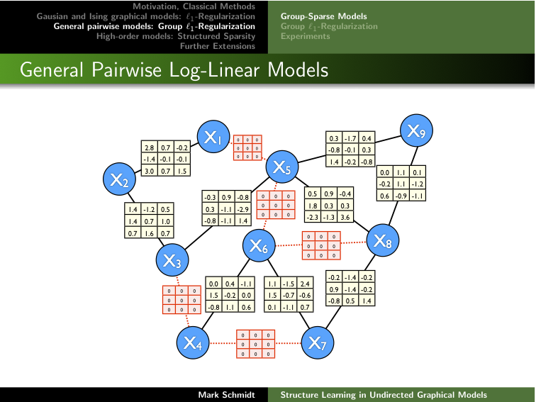
Chapter 5: UGMlearn
This is a new version of the UGMlearn code for structure learning in discrete, pairwise undirected graphical models (UGMs) using group L1-regularization. The main difference between the old code is that this new code is specialized to the case of Markov random fields (unconditional log-linear models), rather than conditional random fields (log-linear models with covariates). Thus, for Markov random fields, it is substantially faster. The new code also includes the ability to use the nuclear norm to encourage low-rank log-potential matrices (for data sets with a large number of states), and makes it easier to allow blockwise-sparse models (or any other grouping of the parameters).
Usage
There are two main functions, LLM2_train and LLM2_trainActive. The active version uses an active-set strategy (as described in Chapters 2-3) to reduce the computation when the graph is sparse, while the non-active version simply uses all variables on all iterations.
The interface to the non-active function is:
>> model = LLM2_train(X,options);
The active case is analogous.
The first input argument, X, contains the training data; element X(s,n) contains the state for variable n in sample s, which must be a positive number between 1 and the maximum number of states. Note that the maximum number of states is taken to be the maximum value of X, and is assumed the same across variables.
The second input argument, options, is a structure that specifies the parameters of the training procedure.
For any field that is not specified, the default is used.
The possible fields that the options structure can include are:
- param: The parameterization of the log-linear model. Use 'I' for Ising, 'P' for generalized Ising, and 'F' for full (see Section 1.5 of the thesis for details). The default is 'F'.
- retype: The type of regularization. Use '2' for L2-regularization, '1' for L1-regularization, 'G' for group L1-regularization with the L2-norm, 'I' for group L1-regularization with the infinity-norm, and 'N' for group L1-regularization with the nuclear-norm. The default is '2'.
- lambda: The regularization strength. The default is 1.
- infer: The type of objective used for training. Use 'exact' to use the exact objective (which is only applicable if the number of nodes and states is very small), use 'pseudo' to use pseudo-likelihood, use 'tree' to use belief propagation on a tree (this only makes sense if the graph structure is actually a tree), use 'mean' to use the Gibbs mean-field free energy after running the mean-field algorithm, use 'loopy' to use the Bethe free energy after running the loopy belief propagation algorithm, and use 'trbp' to use the convexified Bethe free energy after running the tree-reweighted belief propagation algorithm (the weights used for the convexified Bethe use all spanning trees assuming that the graph is full). The default is 'exact'.
- edges: Set this to [] to consider all possible edges. Otherwise, it should contain the list of possible edges to consider. In particular, edges(e,1:2) should contain the numbers of the two nodes associated with the allowed edge e. The default is [].
- useMex: Set this to 1 to allow the use of mex files to speed up parts of the computation in the log-linear model code, and 0 to disable the use of mex files. The default is 1.
- verbose: Set this to 1 to turn on showing the trace of the optimizer as it runs, and 0 to disable this output. The default is 0.
The method returns a structure model, that contains the model parameters and can be used to apply the model to data. In particular, you can evaluate the negative log-likelihood of a data set Xtest using the approximation inferTest using:
>> testNLL = model.nll(model,Xtest,inferTest);
Note that Xtest should not have states that were not included in the training data.
The LLM2_train and LLM2_trainActive functions can also take a third input argument, which gives an initial model structure that is used for warm-starting the optimization. Note that this model structure must have the same set of allowed edges and the same parameterization.
Examples
The function demo_UGMlearn generates a synthetic data set, and uses the code to train log-linear models with different parameterizations and regularization types (assuming exact inference and a fixed value of the regularization strength). The demo_UGMlearn2 function shows how to use the active set method to train the model for a sequence of values of lambda, using the optional third argument to implement warm-starting. The demo_UGMlearn3 function generates a synthetic data set, and uses the code to train log-linear models with different types of approximations to the likelihood.
Gaussian and Conditional Models
Note that this package only includes code for training unconditional discrete pairwise graphical models.
The results on Gaussian data were done using Ewout van den Berg's code from the
PQN paper, while the
CRF results were done using the old version
of UGMlearn.
Chapter 6: LLM
This is a new set of routines for using overlapping group L1-regularization and a hierarchical search strategy for learning hierarchical log-linear models.
Clicking on the image below opens the slides from a talk on this method:
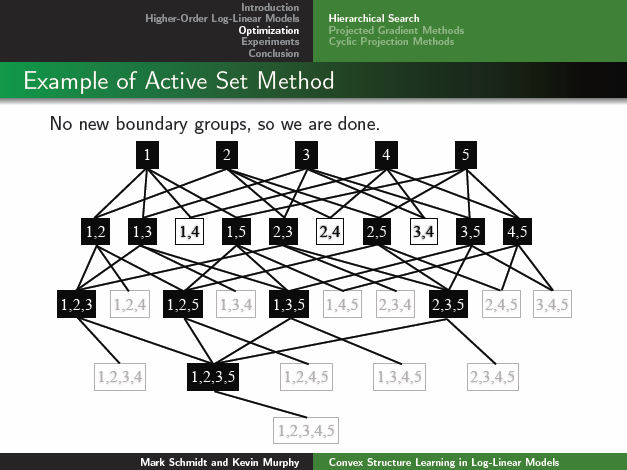
The LLM code extends the LLM2 code from Chapter 5 to allow log-linear factors between up to 7 variables at a time, but the coding was done in a really ugly way.
Usage
The usage is almost identical to the LLM2 code above, except that the functions are named LLM_trainFull for training with all potentials up to fixed order, and LLM_trainGrow for using the hierarchical search. The options structure for these functions can take an extra field order, which specifies the maximum order of the factors (this can be between 2 and 7, and the default is 3). Another difference with the LLM2 is that the default regType parameter is set to 'H', corresponding to the hierarchical group L1-regularization. A third difference with the LLM2 code is that you can not specify the set of allowed edges, right now the code considers all possible edges up to the given order. Finally, note that the LLM code only allows the options 'exact' and 'pseudo' for the infer parameter.
Examples
The function demo_LLM generates a synthetic data set and compares pairwise, threeway, and hierarchical models on the data set. The function demo_LLM2 shows how to use the hierarchical search method to train the model for a sequence of values of lambda, using the optimal third argument for warm-starting.
2012: Update to LLM
In our AIStats 2012 paper "On Sparse, Spectral and Other Parameterizations of Binary Probabilistic Models", we discuss a variety of possible parameterizations of log-linear models. On February 3, 2012, I updated the LLM to include all 5 parameterizations discussed in this work (in the case of binary variables). The function demo_LLM3 generates the same synthetic data set used in demo_LLM, and compares different parameterizations (and regularization strategies) for fitting higher-order models using the active-set method. In some cases, parameterizations that are not discussed in the thesis (in particular, the canonical and spectral parameterizations) give better performance or yield much sparser models that achieve the same level of performance.
2019: Update to Mex File Compilation
In 2019, I updated the "mexAll.m" function to be compatible with the current versions of Matlab, by adding the "-compatibleArrayDims" flag (thanks to Stephen Becker for pointing out this issue).
Download
To use the code, download and unzip thesis.zip.
Then, in Matlab, type:
>> cd thesis             % Change to the relevant directory
>> addpath(genpath(pwd)) % Add all sub-directories to the Matlab path
>> mexAll                % Compile mex files (not necessary on all systems)
>> demo_L1General        % 1st demo of L1General
>> demo_L1Generalpath    % 2nd demo of L1General
>> demo_minConf          % 1st demo of minConf
>> demo_minConfpath      % 2nd demo of minConf
>> demo_DAGlearnGOrdered % 1st demo of DAGlearn
>> demo_DAGlearnG        % 2nd demo of DAGlearn
>> demo_DAGlearn2Ordered % 3rd demo of DAGlearn
>> demo_DAGlearn2        % 4th demo of DAGlearn
>> demo_UGMlearn         % 1st demo of UGMlearn
>> demo_UGMlearn2        % 2nd demo of UGMlearn
>> demo_UGMlearn3        % 3rd demo of UGMlearn
>> demo_LLM              % 1st demo of LLM
>> demo_LLM2             % 2nd demo of LLM
>> demo_LLM3             % 3rd demo of LLM
The latter functions run demos of the functionality of the corresponding packages.