Contents
- Linear Regression on the Simplex
- Lasso regression
- Lasso with Complex Variables
- Group-Sparse Linear Regression with Categorical Features
- Group-Sparse Simultaneous Regression
- Group-Sparse Multinomial Logistic Regression
- Group-Sparse Multi-Task Classification
- Low-Rank Multi-Task Classification
- L_1,inf Blockwise-Sparse Graphical Lasso
- L_1,2 Blockwise-Sparse Graphical Lasso
- Linear Regression with the Over-Lasso
- Kernelized dual form of support vector machines
- Smooth (Primal) Support Vector Machine with Multiple Kernel Learning
- Conditional Random Field Feature Selection
- Approximating node marginals in undirected graphical models with variational mean field
- Multi-State Markov Random Field Structure Learning
- Conditional Random Field Structure Learning with Pseudo-Likelihood
Linear Regression on the Simplex
We will solve min_w |Xw-y|^2, s.t. w >= 0, sum(w)=1
Projection onto the simplex can be computed in O(n log n), this is described in (among other places): Michelot. A Finite Algorithm for Finding the Projection of a Point onto the Canonical Simplex of R^n. Journal of Optimization Theory and Applications (1986).
% Generate Syntehtic Data
nInstances = 50;
nVars = 10;
X = randn(nInstances,nVars);
w = rand(nVars,1).*(rand(nVars,1) > .5);
y = X*w + randn(nInstances,1);

% Initial guess of parameters
wSimplex = zeros(nVars,1);

% Set up Objective Function
funObj = @(w)SquaredError(w,X,y);

% Set up Simplex Projection Function
funProj = @(w)projectSimplex(w);

% Solve with PQN
fprintf('\nComputing optimal linear regression parameters on the simplex...\n');
wSimplex = minConf_PQN(funObj,wSimplex,funProj);

% Check if variable lie in simplex
wSimplex'
fprintf('Min value of wSimplex: %.3f\n',min(wSimplex));
fprintf('Max value of wSimplex: %.3f\n',max(wSimplex));
fprintf('Sum of wSimplex: %.3f\n',sum(wSimplex));
pause
Computing optimal linear regression parameters on the simplex...
 Iteration   FunEvals Projections     Step Length    Function Val        Opt Cond
         1          2          4     2.92731e-03     1.04820e+02     8.97365e-01
         2          3         14     1.00000e+00     6.71088e+01     5.65136e-01
         3          4         22     1.00000e+00     6.70715e+01     2.00314e-01
         4          5         30     1.00000e+00     6.70711e+01     2.61336e-03
         5          6         35     1.00000e+00     6.70711e+01     1.01669e-04
Directional Derivative below progTol

ans =

  Columns 1 through 7

    0.2474         0         0    0.2932    0.4594         0         0

  Columns 8 through 10

         0         0         0

Min value of wSimplex: 0.000
Max value of wSimplex: 0.459
Sum of wSimplex: 1.000
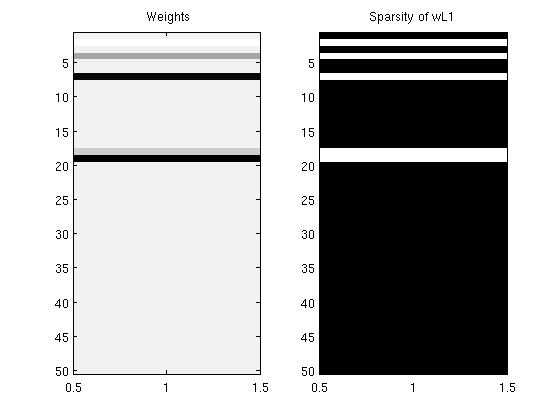
Lasso regression
We will solve min_w |Xw-y|^2 s.t. sum_i w_i <= tau
Projection onto the L1-Ball can be computed in O(n), see: Duchi, Shalev-Schwartz, Singer, and Chandra. Efficient Projections onto the L1-Ball for Learning in High Dimensions. ICML (2008).
% Generate Syntehtic Data
nInstances = 500;
nVars = 50;
X = randn(nInstances,nVars);
w = randn(nVars,1).*(rand(nVars,1) > .5);
y = X*w + randn(nInstances,1);

% Initial guess of parameters
wL1 = zeros(nVars,1);

% Set up Objective Function
funObj = @(w)SquaredError(w,X,y);

% Set up L1-Ball Projection
tau = 2;
funProj = @(w)sign(w).*projectRandom2C(abs(w),tau);

% Solve with PQN
fprintf('\nComputing optimal Lasso parameters...\n');
wL1 = minConf_PQN(funObj,wL1,funProj);
wL1(abs(wL1) < 1e-4) = 0;

% Check sparsity of solution
wL1'
fprintf('Number of non-zero variables in solution: %d (of %d)\n',nnz(wL1),length(wL1));

figure;
subplot(1,2,1);
imagesc(wL1);colormap gray;
title(' Weights');
subplot(1,2,2);
imagesc(wL1~=0);colormap gray;
title('Sparsity of wL1');
pause
Computing optimal Lasso parameters...
 Iteration   FunEvals Projections     Step Length    Function Val        Opt Cond
         1          2          4     3.69062e-05     1.58865e+04     1.99993e+00
         2          3         15     1.00000e+00     1.19915e+04     1.29253e+00
         3          4         24     1.00000e+00     1.19883e+04     1.23647e+00
         4          5         32     1.00000e+00     1.19882e+04     2.62204e-01
         5          6         39     1.00000e+00     1.19882e+04     3.76125e-02
         6          7         45     1.00000e+00     1.19882e+04     1.08715e-03
Directional Derivative below progTol

ans =

  Columns 1 through 7

         0    0.0526         0   -0.2532         0         0   -0.7711

  Columns 8 through 14

         0         0         0         0         0         0         0

  Columns 15 through 21

         0         0         0   -0.1177   -0.8054         0         0

  Columns 22 through 28

         0         0         0         0         0         0         0

  Columns 29 through 35

         0         0         0         0         0         0         0

  Columns 36 through 42

         0         0         0         0         0         0         0

  Columns 43 through 49

         0         0         0         0         0         0         0

  Column 50

         0

Number of non-zero variables in solution: 5 (of 50)
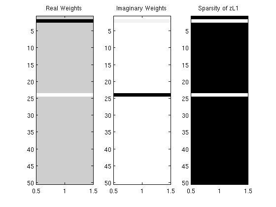
Lasso with Complex Variables
We will solve min_w |Xz-y|^2, s.t. sum_i z_i <= tau, where z and y are complex, and z represents the complex modulus
Efficient projection onto this complex L1-Ball is described in: van den Berg and Friedlander. Probing the Pareto Frontier for Basis Pursuit Solutions. SIAM Journal of Scientific Computing (2008).
The calculation of the projection can be reduced from the O(n log n) required in the above to O(n) by using a linear-time median finding algorithm
% Generate Syntehtic Data
nInstances = 500;
nVars = 50;
X = randn(nInstances,nVars);
z = complex(randn(nVars,1),randn(nVars,1)).*(rand(nVars,1) > .5);
y = X*z;

% Initial guess of parameters
zReal = zeros(nVars,1);
zImag = zeros(nVars,1);

% Set up Objective Function
funObj = @(zRealImag)SquaredError(zRealImag,[X zeros(nInstances,nVars);zeros(nInstances,nVars) X],[real(y);imag(y)]);

% Set up Complex L1-Ball Projection
tau = 2;
funProj = @(zRealImag)complexProject(zRealImag,tau);

% Solve with PQN
fprintf('\nComputing optimal Lasso parameters...\n');
zRealImag = minConf_PQN(funObj,[zReal;zImag],funProj);
zReal = zRealImag(1:nVars);
zImag = zRealImag(nVars+1:end);
zL1 = complex(zReal,zImag);
zL1(abs(zL1) < 1e-4) = 0;

figure
subplot(1,3,1);
imagesc(zReal);colormap gray;
title('Real Weights');
subplot(1,3,2);
imagesc(zImag);colormap gray;
title('Imaginary Weights');
subplot(1,3,3);
imagesc(zL1~=0);colormap gray;
title('Sparsity of zL1');

% Check sparsity of solution
zL1'
fprintf('Number of non-zero variables in solution: %d (of %d)\n',nnz(zL1),length(zL1));
pause
Computing optimal Lasso parameters...
 Iteration   FunEvals Projections     Step Length    Function Val        Opt Cond
         1          2          4     2.48486e-05     2.25735e+04     1.99850e+00
         2          3         13     1.00000e+00     1.72665e+04     7.89444e-01
         3          4         20     1.00000e+00     1.72652e+04     1.24561e+00
         4          5         27     1.00000e+00     1.72652e+04     1.25796e-02
         5          6         33     1.00000e+00     1.72652e+04     2.99222e-04
Directional Derivative below progTol

ans =

  Columns 1 through 4

        0            -1.2442 + 0.0335i        0                  0

  Columns 5 through 8

        0                  0                  0                  0

  Columns 9 through 12

        0                  0                  0                  0

  Columns 13 through 16

        0                  0                  0                  0

  Columns 17 through 20

        0                  0                  0                  0

  Columns 21 through 24

        0                  0                  0             0.2936 + 0.6959i

  Columns 25 through 28

        0                  0                  0                  0

  Columns 29 through 32

        0                  0                  0                  0

  Columns 33 through 36

        0                  0                  0                  0

  Columns 37 through 40

        0                  0                  0                  0

  Columns 41 through 44

        0                  0                  0                  0

  Columns 45 through 48

        0                  0                  0                  0

  Columns 49 through 50

        0                  0

Number of non-zero variables in solution: 2 (of 50)
Group-Sparse Linear Regression with Categorical Features
We will solve min_w |Xw-y|^2, s.t. sum_g |w_g|_inf <= tau, where X uses binary indicator variables to represent a set of categorical features, and we use the 'groups' g to encourage sparsity in terms of the original categorical variables
Using the L_1,inf mixed-norm for group-sparsity is described in: Turlach, Venables, and Wright. Simultaneous Variable Selection. Technometrics (2005).
Using group sparsity to select for categorical variables encoded with indicator variables is described in: Yuan and Lin. Model Selection and Estimation in Regression with Grouped Variables. JRSSB (2006).
Projection onto the L_1,inf mixed-norm ball can be computed in O(n log n), this is described in: Quattoni, Carreras, Collins, and Darell. An Efficient Projection for l_{1,\infty} Regularization. ICML (2009).
% Generate categorical features
nInstances = 100;
nStates = [3 3 3 3 5 4 5 5 6 10 3]; % Number of discrete states for each categorical feature
X = zeros(nInstances,length(nStates));
offset = 0;
for i = 1:nInstances
    for s = 1:length(nStates)
        prob_s = rand(nStates(s),1);
        prob_s = prob_s/sum(prob_s);
        X(i,s) = sampleDiscrete(prob_s);
    end
end

% Make indicator variable encoding of categorical features
X_ind = zeros(nInstances,sum(nStates));
clear w
for s = 1:length(nStates)
    for i = 1:nInstances
        X_ind(i,offset+X(i,s)) = 1;
    end
    w(offset+1:offset+nStates(s),1) = (rand > .75)*randn(nStates(s),1);
    offset = offset+nStates(s);
end
y = X_ind*w + randn(nInstances,1);

% Initial guess of parameters
w_ind = zeros(sum(nStates),1);

% Set up Objective Function
funObj = @(w)SquaredError(w,X_ind,y);

% Set up groups
offset = 0;
groups = zeros(size(w_ind));
for s = 1:length(nStates)
    groups(offset+1:offset+nStates(s),1) = s;
    offset = offset+nStates(s);
end

% Set up L_1,inf Projection Function
tau = .05;
funProj = @(w)groupLinfProj(w,tau,groups);

% Solve with PQN
fprintf('\nComputing Group-Sparse Linear Regression with Categorical Features Parameters...\n');
w_ind = minConf_PQN(funObj,w_ind,funProj);
w_ind(abs(w_ind) < 1e-4) = 0;

% Check selected variables
w_ind'
for s = 1:length(nStates)
   fprintf('Number of non-zero variables associated with categorical variable %d: %d (of %d)\n',s,nnz(w_ind(groups==s)),sum(groups==s));
end
fprintf('Total number of categorical variables selected: %d (of %d)\n',nnz(accumarray(groups,abs(w_ind))),length(nStates));
pause
Computing Group-Sparse Linear Regression with Categorical Features Parameters...
 Iteration   FunEvals Projections     Step Length    Function Val        Opt Cond
         1          2          4     6.75309e-04     4.02268e+02     4.99662e-02
         2          3          9     1.00000e+00     3.88459e+02     0.00000e+00
First-Order Optimality Conditions Below optTol

ans =

  Columns 1 through 7

         0         0         0         0         0         0         0

  Columns 8 through 14

         0         0   -0.0500    0.0500    0.0500         0         0

  Columns 15 through 21

         0         0         0         0         0         0         0

  Columns 22 through 28

         0         0         0         0         0         0         0

  Columns 29 through 35

         0         0         0         0         0         0         0

  Columns 36 through 42

         0         0         0         0         0         0         0

  Columns 43 through 49

         0         0         0         0         0         0         0

  Column 50

         0

Number of non-zero variables associated with categorical variable 1: 0 (of 3)
Number of non-zero variables associated with categorical variable 2: 0 (of 3)
Number of non-zero variables associated with categorical variable 3: 0 (of 3)
Number of non-zero variables associated with categorical variable 4: 3 (of 3)
Number of non-zero variables associated with categorical variable 5: 0 (of 5)
Number of non-zero variables associated with categorical variable 6: 0 (of 4)
Number of non-zero variables associated with categorical variable 7: 0 (of 5)
Number of non-zero variables associated with categorical variable 8: 0 (of 5)
Number of non-zero variables associated with categorical variable 9: 0 (of 6)
Number of non-zero variables associated with categorical variable 10: 0 (of 10)
Number of non-zero variables associated with categorical variable 11: 0 (of 3)
Total number of categorical variables selected: 1 (of 11)
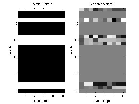
Group-Sparse Simultaneous Regression
We will solve min_W |XW-Y|^2 + lambda * sum_g |W_g|_inf, where we use the 'groups' g to encourage that we select variables that are relevant across the output variables
We solve this non-differentiable problem by transforming it into the equivalent problem: min_w |XW-Y|^2 + lambda * sum_g alpha_g, s.t. forall_g alpha_g >= |W_g|_inf
Using group-sparsity to select variables that are relevant across regression tasks is described in: Turlach, Venables, and Wright. Simultaneous Variable Selection. Technometrics (2005).
The auxiliary variable formulation is described in: Schmidt, Murphy, Fung, and Rosales. Structure Learning in Random Field for Heart Motion Abnormality Detection. CVPR (2008).
Computing the projection in the auxiliary variable formulation can be done in O(n log n), this is described in the addendum of the above paper.
% Generate synthetic data
nInstances = 100;
nVars = 25;
nOutputs = 10;
X = randn(nInstances,nVars);
W = diag(rand(nVars,1) > .75)*randn(nVars,nOutputs);
Y = X*W + randn(nInstances,nOutputs);

% Initial guess of parameters
W_groupSparse = zeros(nVars,nOutputs);

% Set up Objective Function
funObj = @(W)SimultaneousSquaredError(W,X,Y);

% Set up Groups
groups = repmat([1:nVars]',1,nOutputs);
groups = groups(:);
nGroups = max(groups);

% Initialize auxiliary variables that will bound norm
lambda = 250;
alpha = zeros(nGroups,1);
penalizedFunObj = @(W)auxGroupLoss(W,groups,lambda,funObj);

% Set up L_1,inf Projection Function
[groupStart,groupPtr] = groupl1_makeGroupPointers(groups);
funProj = @(W)auxGroupLinfProject(W,nVars*nOutputs,groupStart,groupPtr);

% Solve with PQN
fprintf('\nComputing group-sparse simultaneous regression parameters...\n');
Walpha = minConf_PQN(penalizedFunObj,[W_groupSparse(:);alpha],funProj);

% Extract parameters from augmented vector
W_groupSparse(:) = Walpha(1:nVars*nOutputs);
W_groupSparse(abs(W_groupSparse) < 1e-4) = 0;

figure
subplot(1,2,1);
imagesc(W_groupSparse~=0);colormap gray
title('Sparsity Pattern');
ylabel('variable');
xlabel('output target');
subplot(1,2,2);
imagesc(W_groupSparse);colormap gray
title('Variable weights');
ylabel('variable');
xlabel('output target');

% Check selected variables
for s = 1:nVars
   fprintf('Number of tasks where variable %d was selected: %d (of %d)\n',s,nnz(W_groupSparse(s,:)),nOutputs);
end
fprintf('Total number of variables selected: %d (of %d)\n',nnz(sum(W_groupSparse,2)),nVars);
pause
Computing group-sparse simultaneous regression parameters...
 Iteration   FunEvals Projections     Step Length    Function Val        Opt Cond
         1          2          4     4.22539e-05     7.06280e+03     2.19202e+02
         2          3         16     1.00000e+00     3.15351e+03     2.39651e+01
         3          4         28     1.00000e+00     3.10418e+03     9.86012e+00
         4          5         40     1.00000e+00     3.09330e+03     2.56478e+00
         5          6         52     1.00000e+00     3.09277e+03     9.42922e-01
         6          7         64     1.00000e+00     3.09272e+03     3.99847e-01
         7          8         76     1.00000e+00     3.09272e+03     1.76031e-01
         8          9         88     1.00000e+00     3.09272e+03     4.70416e-02
         9         10         99     1.00000e+00     3.09272e+03     1.24753e-02
        10         11        108     1.00000e+00     3.09272e+03     3.95741e-03
        11         12        115     1.00000e+00     3.09272e+03     5.25340e-04
        12         13        121     1.00000e+00     3.09272e+03     2.60962e-04
Directional Derivative below progTol
Number of tasks where variable 1 was selected: 10 (of 10)
Number of tasks where variable 2 was selected: 0 (of 10)
Number of tasks where variable 3 was selected: 0 (of 10)
Number of tasks where variable 4 was selected: 10 (of 10)
Number of tasks where variable 5 was selected: 0 (of 10)
Number of tasks where variable 6 was selected: 0 (of 10)
Number of tasks where variable 7 was selected: 0 (of 10)
Number of tasks where variable 8 was selected: 0 (of 10)
Number of tasks where variable 9 was selected: 10 (of 10)
Number of tasks where variable 10 was selected: 10 (of 10)
Number of tasks where variable 11 was selected: 10 (of 10)
Number of tasks where variable 12 was selected: 0 (of 10)
Number of tasks where variable 13 was selected: 0 (of 10)
Number of tasks where variable 14 was selected: 0 (of 10)
Number of tasks where variable 15 was selected: 0 (of 10)
Number of tasks where variable 16 was selected: 0 (of 10)
Number of tasks where variable 17 was selected: 0 (of 10)
Number of tasks where variable 18 was selected: 0 (of 10)
Number of tasks where variable 19 was selected: 0 (of 10)
Number of tasks where variable 20 was selected: 0 (of 10)
Number of tasks where variable 21 was selected: 0 (of 10)
Number of tasks where variable 22 was selected: 0 (of 10)
Number of tasks where variable 23 was selected: 10 (of 10)
Number of tasks where variable 24 was selected: 10 (of 10)
Number of tasks where variable 25 was selected: 0 (of 10)
Total number of variables selected: 7 (of 25)
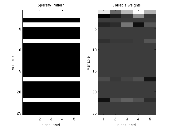
Group-Sparse Multinomial Logistic Regression
We will solve min_W nll(W,X,y) + lambda * sum_g |W_g|_2, where nll(W,X,y) is the negative log-likelihood in multinomial logistic regression, and where we use the 'groups' g to encourage sparsity in terms of the original input variables
We solve this non-differentiable problem by transforming it into the equivalent problem: min_W nll(W,X,y) + lambda * sum_g alpha_g, s.t. forall_g alpha_g >= |W_g|_2
Note: the bias variables are assigned to group '0', which is not penalized
Using the L_1,2 mixed-norm for group-sparsity is described in: Bakin. Adaptive Regression and Model Selection in Data Mining Problems. PhD Thesis Australian National University (1999)
Using group-sparsity to select the original input variables in multinomial classification is described in: Obozinski, Taskar, and Jordan. Joint covariate selection for grouped classification. UC Berkeley TR (2007).
The auxiliary variable formulation is described in the addendum of: Schmidt, Murphy, Fung, and Rosales. Structure Learning in Random Field for Heart Motion Abnormality Detection. CVPR (2008).
Computing the projection in the auxiliary variable formulation can be done in O(n), this is Exercise 8.3(c) of: Boyd and Vandenberghe. Convex Optimization. Cambridge University Press (2004).
% Generate synthetic data
nInstances = 100;
nVars = 25;
nClasses = 6;
X = [ones(nInstances,1) randn(nInstances,nVars-1)];
W = diag(rand(nVars,1) > .75)*randn(nVars,nClasses);
[junk y] = max(X*W + randn(nInstances,nClasses),[],2);

% Initial guess of parameters
W_groupSparse = zeros(nVars,nClasses-1);

% Set up Objective Function
funObj = @(W)SoftmaxLoss2(W,X,y,nClasses);

% Set up Groups (don't penalized bias)
groups = [zeros(1,nClasses-1);repmat([1:nVars-1]',1,nClasses-1)];
groups = groups(:);
nGroups = max(groups);

% Initialize auxiliary variables that will bound norm
lambda = 10;
alpha = zeros(nGroups,1);
penalizedFunObj = @(W)auxGroupLoss(W,groups,lambda,funObj);

% Set up L_1,2 Projection Function
[groupStart,groupPtr] = groupl1_makeGroupPointers(groups);
funProj = @(W)auxGroupL2Project(W,nVars*(nClasses-1),groupStart,groupPtr);

% Solve with PQN
fprintf('\nComputing group-sparse multinomial logistic regression parameters...\n');
Walpha = minConf_PQN(penalizedFunObj,[W_groupSparse(:);alpha],funProj);

% Extract parameters from augmented vector
W_groupSparse(:) = Walpha(1:nVars*(nClasses-1));
W_groupSparse(abs(W_groupSparse) < 1e-4) = 0;

figure
subplot(1,2,1);
imagesc(W_groupSparse~=0);colormap gray
title('Sparsity Pattern');
ylabel('variable');
xlabel('class label');
subplot(1,2,2);
imagesc(W_groupSparse);colormap gray
title('Variable weights');
ylabel('variable');
xlabel('class label');

% Check selected variables
fprintf('Number of classes where bias variable was selected: %d (of %d)\n',nnz(W_groupSparse(1,:)),nClasses-1);
for s = 2:nVars
   fprintf('Number of classes where variable %d was selected: %d (of %d)\n',s,nnz(W_groupSparse(s,:)),nClasses-1);
end
fprintf('Total number of variables selected: %d (of %d)\n',nnz(sum(W_groupSparse(2:end,:),2)),nVars);
pause
Computing group-sparse multinomial logistic regression parameters...
 Iteration   FunEvals Projections     Step Length    Function Val        Opt Cond
         1          2          4     1.29290e-03     1.77636e+02     1.70112e+01
         2          3         16     1.00000e+00     1.35096e+02     5.41046e+00
         3          4         28     1.00000e+00     1.31176e+02     2.49132e+00
         4          5         40     1.00000e+00     1.30339e+02     1.17206e+00
         5          6         52     1.00000e+00     1.29858e+02     1.49862e+00
         6          7         64     1.00000e+00     1.29415e+02     1.00392e+00
         7          8         76     1.00000e+00     1.28789e+02     7.82402e-01
         8          9         87     1.00000e+00     1.28472e+02     1.55317e+00
         9         10         99     1.00000e+00     1.28259e+02     5.06381e-01
        10         11        110     1.00000e+00     1.28203e+02     2.35309e-01
        11         12        121     1.00000e+00     1.28180e+02     1.70284e-01
        12         13        132     1.00000e+00     1.28173e+02     7.28148e-02
        13         14        143     1.00000e+00     1.28170e+02     3.66599e-02
        14         15        153     1.00000e+00     1.28170e+02     1.09387e-02
        15         16        163     1.00000e+00     1.28169e+02     1.22609e-02
        16         18        174     3.59127e-01     1.28169e+02     6.22380e-03
        17         19        186     1.00000e+00     1.28169e+02     2.73340e-03
        18         20        197     1.00000e+00     1.28169e+02     2.83436e-03
        19         21        208     1.00000e+00     1.28169e+02     4.79012e-03
        20         22        219     1.00000e+00     1.28169e+02     1.02580e-03
        21         23        230     1.00000e+00     1.28169e+02     1.90541e-04
        22         24        241     1.00000e+00     1.28169e+02     2.52536e-04
        23         25        253     1.00000e+00     1.28169e+02     6.74493e-05
Directional Derivative below progTol
Number of classes where bias variable was selected: 5 (of 5)
Number of classes where variable 2 was selected: 5 (of 5)
Number of classes where variable 3 was selected: 0 (of 5)
Number of classes where variable 4 was selected: 5 (of 5)
Number of classes where variable 5 was selected: 0 (of 5)
Number of classes where variable 6 was selected: 0 (of 5)
Number of classes where variable 7 was selected: 0 (of 5)
Number of classes where variable 8 was selected: 5 (of 5)
Number of classes where variable 9 was selected: 0 (of 5)
Number of classes where variable 10 was selected: 0 (of 5)
Number of classes where variable 11 was selected: 0 (of 5)
Number of classes where variable 12 was selected: 0 (of 5)
Number of classes where variable 13 was selected: 0 (of 5)
Number of classes where variable 14 was selected: 0 (of 5)
Number of classes where variable 15 was selected: 0 (of 5)
Number of classes where variable 16 was selected: 0 (of 5)
Number of classes where variable 17 was selected: 5 (of 5)
Number of classes where variable 18 was selected: 0 (of 5)
Number of classes where variable 19 was selected: 0 (of 5)
Number of classes where variable 20 was selected: 0 (of 5)
Number of classes where variable 21 was selected: 0 (of 5)
Number of classes where variable 22 was selected: 5 (of 5)
Number of classes where variable 23 was selected: 0 (of 5)
Number of classes where variable 24 was selected: 0 (of 5)
Number of classes where variable 25 was selected: 0 (of 5)
Total number of variables selected: 5 (of 25)
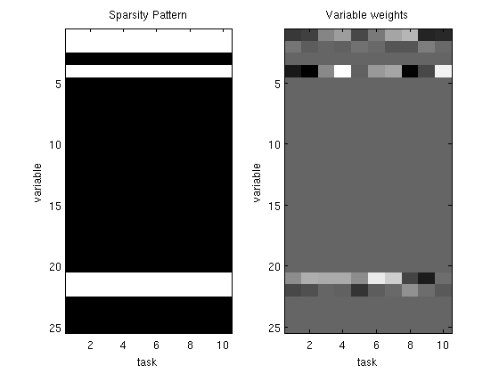
Group-Sparse Multi-Task Classification
We will solve min_W nll(W,X,Y), s.t. sum_g |W_g|_2 <= tau, where nll(W,X,Y) is the negative log-likelihood in a simultaneous binary logistic regression model, and where we use the 'groups' g to encourage that we select variables that are relevant across the binary classification tasks
Note: the bias variables are assigned to group '0', which is not penalized
Using group-sparsity to select variables that are relevant across classification tasks is described in: Obozinski, Taskar, and Jordan. Joint covariate selection for grouped classification. UC Berkeley TR (2007).
Projection onto the L_1,2 mixed-norm ball can be computed in O(n), this is described in: van den Berg, Schmidt, Friedlander, and Murphy. Group Sparsity via Linear-Time Projection. UBC TR (2008).
% Generate synthetic data
nInstances = 100;
nVars = 25;
nOutputs = 10;
X = [ones(nInstances,1) randn(nInstances,nVars-1)];
W = diag(rand(nVars,1) > .75)*randn(nVars,nOutputs);
Y = X*W + randn(nInstances,nOutputs);

% Initial guess of parameters
W_groupSparse = zeros(nVars,nOutputs);

% Set up Objective Function
funObj = @(W)SimultaneousLogisticLoss(W,X,Y);

% Set up Groups (don't penalized bias)
groups = [zeros(1,nOutputs);repmat([1:nVars-1]',1,nOutputs)];
groups = groups(:);
nGroups = max(groups);

% Set up L_1,2 Projection Function
tau = .5;
funProj = @(W)groupL2Proj(W,tau,groups);

% Solve with PQN
fprintf('\nComputing Group-Sparse Multi-Task Classification Parameters...\n');
W_groupSparse(:) = minConf_PQN(funObj,W_groupSparse(:),funProj);
W_groupSparse(abs(W_groupSparse) < 1e-4) = 0;

figure
subplot(1,2,1);
imagesc(W_groupSparse~=0);colormap gray
title('Sparsity Pattern');
ylabel('variable');
xlabel('task');
subplot(1,2,2);
imagesc(W_groupSparse);colormap gray
title('Variable weights');
ylabel('variable');
xlabel('task');

% Check selected variables
fprintf('Number of classes where bias variable was selected: %d (of %d)\n',nnz(W_groupSparse(1,:)),nOutputs);
for s = 2:nVars
   fprintf('Number of tasks where variable %d was selected: %d (of %d)\n',s,nnz(W_groupSparse(s,:)),nOutputs);
end
fprintf('Total number of variables selected: %d (of %d)\n',nnz(sum(W_groupSparse(2:end,:),2)),nVars);
pause
Computing Group-Sparse Multi-Task Classification Parameters...
 Iteration   FunEvals Projections     Step Length    Function Val        Opt Cond
         1          2          4     1.63146e-04     6.92877e+02     2.25943e+01
         2          3         16     1.00000e+00     6.01621e+02     4.46004e+00
         3          4         28     1.00000e+00     6.00586e+02     3.56626e+00
         4          5         40     1.00000e+00     6.00077e+02     1.99417e+00
         5          6         52     1.00000e+00     5.99967e+02     6.37449e-01
         6          7         64     1.00000e+00     5.99963e+02     1.96763e-01
         7          8         75     1.00000e+00     5.99963e+02     5.62389e-02
         8          9         87     1.00000e+00     5.99963e+02     2.11416e-02
         9         10         97     1.00000e+00     5.99963e+02     3.10355e-03
        10         11        104     1.00000e+00     5.99963e+02     8.99030e-04
        11         12        111     1.00000e+00     5.99963e+02     1.33924e-04
Directional Derivative below progTol
Number of classes where bias variable was selected: 10 (of 10)
Number of tasks where variable 2 was selected: 10 (of 10)
Number of tasks where variable 3 was selected: 0 (of 10)
Number of tasks where variable 4 was selected: 10 (of 10)
Number of tasks where variable 5 was selected: 0 (of 10)
Number of tasks where variable 6 was selected: 0 (of 10)
Number of tasks where variable 7 was selected: 0 (of 10)
Number of tasks where variable 8 was selected: 0 (of 10)
Number of tasks where variable 9 was selected: 0 (of 10)
Number of tasks where variable 10 was selected: 0 (of 10)
Number of tasks where variable 11 was selected: 0 (of 10)
Number of tasks where variable 12 was selected: 0 (of 10)
Number of tasks where variable 13 was selected: 0 (of 10)
Number of tasks where variable 14 was selected: 0 (of 10)
Number of tasks where variable 15 was selected: 0 (of 10)
Number of tasks where variable 16 was selected: 0 (of 10)
Number of tasks where variable 17 was selected: 0 (of 10)
Number of tasks where variable 18 was selected: 0 (of 10)
Number of tasks where variable 19 was selected: 0 (of 10)
Number of tasks where variable 20 was selected: 0 (of 10)
Number of tasks where variable 21 was selected: 10 (of 10)
Number of tasks where variable 22 was selected: 10 (of 10)
Number of tasks where variable 23 was selected: 0 (of 10)
Number of tasks where variable 24 was selected: 0 (of 10)
Number of tasks where variable 25 was selected: 0 (of 10)
Total number of variables selected: 4 (of 25)
Low-Rank Multi-Task Classification
We will solve min_W nll(W,X,Y) s.t. |W|_sigma <= tau, where nll(W,X,Y) is the negative log-likelihood in a simultaneous binary logistic regression model, and where the nuclear norm |W|_sigma encourages W to be low-rank
W = zeros(nVars,nOutputs);
funProj = @(w)traceProject(w,nVars,tau);

fprintf('\nComputing Low-Rank Multi-Task Classification Parameters...\n');
W(:) = minConf_PQN(funObj,W(:),funProj);

s = svd(W);

fprintf('Number of non-zero singular values: %d (of %d)\n',sum(s > 1e-4),length(s));
pause
Computing Low-Rank Multi-Task Classification Parameters...
 Iteration   FunEvals Projections     Step Length    Function Val        Opt Cond
         1          2          4     1.63146e-04     6.93116e+02     1.72961e-01
         2          3         16     1.00000e+00     5.73676e+02     1.24511e-01
         3          4         28     1.00000e+00     5.71969e+02     1.10654e-01
         4          5         40     1.00000e+00     5.71629e+02     1.02558e-01
         5          6         52     1.00000e+00     5.71608e+02     8.05868e-02
         6          7         64     1.00000e+00     5.71608e+02     4.08470e-02
         7          8         75     1.00000e+00     5.71608e+02     1.54377e-02
         8          9         84     1.00000e+00     5.71608e+02     2.05653e-03
         9         10         92     1.00000e+00     5.71608e+02     9.97128e-04
        10         11        100     1.00000e+00     5.71608e+02     1.28489e-04
Directional Derivative below progTol
Number of non-zero singular values: 3 (of 10)
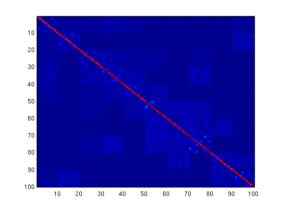
L_1,inf Blockwise-Sparse Graphical Lasso
We will solve nll(K,S) + sum_b lambda_b||K_b||_inf, where nll(K,S) is the Gaussian negative log-likelihood and the 'blocks' b encourage blockwise sparsity in the matrix between 'groups' g
We solve this non-differentiable problem by solving the convex dual problem: min_W -logdet(S + W), s.t. sum_b |W_b|_inf <= lambda
Using the L_1,inf mixed-norm to encourage blockwise sparsity, and the derivation of the convex dual problem are described in: Duchi, Gould, and Koller. Projected Subgradient Methods for Learning Sparse Gaussians. UAI (2008).
% Generate a set of variable groups
nNodes = 100;
nGroups = 10;
groups = repmat(1:nNodes/nGroups,nGroups,1);
groups = groups(:);

% Generate a positive-definite matrix that is sparse within groups, and
% blockwise sparse between groups
betweenSparsity = (rand(nGroups) > .75).*triu(ones(nGroups),1);
adj = triu(randn(nNodes).*(rand(nNodes) > .1),1);
for g1 = 1:nGroups
    for g2 = g1+1:nGroups
        if betweenSparsity(g1,g2) == 0
           adj(groups==g1,groups==g2) = 0;
        end
    end
end
adj = adj+adj';
tau = 1;
invCov = adj + tau*eye(nNodes);
while ~ispd(invCov)
    tau = tau*2;
    invCov = adj + tau*eye(nNodes);
end
mu = randn(nNodes,1);

% Sample from the GGM
nInstances = 500;
C = inv(invCov);
R = chol(C)';
X = zeros(nInstances,nNodes);
for i = 1:nInstances
   X(i,:) = (mu + R*randn(nNodes,1))';
end

% Center and Standardize
X = standardizeCols(X);

% Compute empirical covariance
S = cov(X);

% Set up Objective Function
funObj = @(K)logdetFunction(K,S);

% Set up Weights on penalty (multiply lambda by number of elements in
% block)
lambda = 10/nInstances;
for g = 1:nGroups
    nBlockElements(g,1) = sum(groups==g);
end
lambdaBlock = setdiag(lambda * nBlockElements*nBlockElements',lambda);

lambdaBlock = lambdaBlock(:);
funProj = @(K)projectLinf1(K,nNodes,nBlockElements,lambdaBlock);

% Initial guess of parameters
W = lambda*eye(nNodes);

% Solve with PQN
fprintf('\nComputing L_1,inf Blockwise-Sparse Graphical Lasso Parameters...\n');
W(:) = minConf_PQN(funObj,W(:),funProj);
K = inv(S+W);

figure
imagesc(abs(K))
pause
Computing L_1,inf Blockwise-Sparse Graphical Lasso Parameters...
 Iteration   FunEvals Projections     Step Length    Function Val        Opt Cond
         1          2          4     1.33147e-03     1.54715e+01     3.07292e-01
         2          3         16     1.00000e+00     7.30547e+00     9.08283e-02
         3          4         28     1.00000e+00     4.41716e+00     3.31314e-02
         4          5         40     1.00000e+00     3.95820e+00     2.07873e-02
         5          6         52     1.00000e+00     3.88628e+00     8.89573e-03
         6          7         64     1.00000e+00     3.87674e+00     3.58001e-03
         7          8         76     1.00000e+00     3.87530e+00     1.98297e-03
         8          9         88     1.00000e+00     3.87506e+00     5.66522e-04
         9         10        100     1.00000e+00     3.87499e+00     3.09082e-04
        10         11        112     1.00000e+00     3.87498e+00     4.65249e-04
        11         12        124     1.00000e+00     3.87498e+00     7.38526e-05
        12         13        135     1.00000e+00     3.87498e+00     5.38388e-05
        13         14        147     1.00000e+00     3.87498e+00     3.69698e-05
        14         15        159     1.00000e+00     3.87498e+00     3.32326e-05
        15         16        165     1.00000e+00     3.87498e+00     4.06379e-06
First-Order Optimality Conditions Below optTol
L_1,2 Blockwise-Sparse Graphical Lasso
Same as the above, but we use the L_1,2 group-norm instead of L_1,inf, as discussed in the PQN paper.
lambdaBlock = lambdaBlock/5;
funProj = @(K)projectLinf2(K,nNodes,nBlockElements,lambdaBlock);

% Initial guess of parameters
W = lambda*eye(nNodes);

% Solve with PQN
fprintf('\nComputing L_1,2 Blockwise-Sparse Graphical Lasso Parameters...\n');
W(:) = minConf_PQN(funObj,W(:),funProj);
K = inv(S+W);

figure
imagesc(abs(K))
pause
Computing L_1,2 Blockwise-Sparse Graphical Lasso Parameters...
 Iteration   FunEvals Projections     Step Length    Function Val        Opt Cond
         1          2          4     1.26362e-03     1.77151e+01     1.58734e-01
         2          3         16     1.00000e+00     9.52799e+00     9.38708e-02
         3          4         28     1.00000e+00     5.75888e+00     5.11887e-02
         4          5         40     1.00000e+00     5.04321e+00     2.54468e-02
         5          6         52     1.00000e+00     4.90755e+00     1.72770e-02
         6          7         64     1.00000e+00     4.88031e+00     8.38630e-03
         7          8         76     1.00000e+00     4.87530e+00     4.83360e-03
         8          9         88     1.00000e+00     4.87421e+00     2.13371e-03
         9         10        100     1.00000e+00     4.87371e+00     7.76676e-04
        10         11        112     1.00000e+00     4.87359e+00     2.33940e-03
        11         12        124     1.00000e+00     4.87355e+00     4.84442e-04
        12         13        136     1.00000e+00     4.87355e+00     1.76255e-04
        13         14        148     1.00000e+00     4.87354e+00     6.12743e-05
        14         15        160     1.00000e+00     4.87354e+00     1.02723e-04
        15         16        172     1.00000e+00     4.87354e+00     4.31139e-05
        16         17        183     1.00000e+00     4.87354e+00     1.02161e-05
        17         18        191     1.00000e+00     4.87354e+00     7.88540e-06
First-Order Optimality Conditions Below optTol

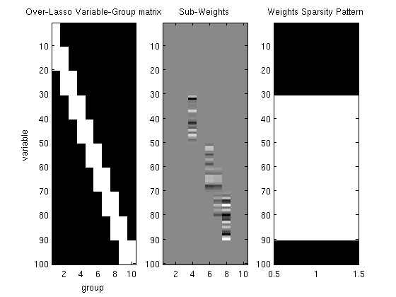
Linear Regression with the Over-Lasso
We will solve the "Over-Lasso" problem: min_w |Xw-Y|^2 + lambda * sum_g |v_g|, s.t. sum v_i = w_i This is similar to the 'group' lasso' problems above, but in this case each variable is represented as a linear combination of 'sub' variables 'v', and these sub variables can belong to different groups. This leads to sparse solutions that tend to be unions of groups
We solve this problem by eliminating w, and using auxiliary variables to make the problem differentiable
The "Over-Lasso" regularizer and the method of eliminating w are described in: Jacob, Obozinski, and Vert. Group Lasso with Overlap and Graph Lasso. ICML (2009).
% Make variable-group membership matrix
nVars = 100;
nGroups = 10;
varGroupMatrix = zeros(nVars,nGroups);
offset = 0;
for g = 1:nGroups
   varGroupMatrix(offset+1:min(offset+2*nVars/nGroups,nVars),g) = 1;
   offset = offset + nVars/nGroups;
end

% Generate synthetic data
nInstances = 250;
X = randn(nInstances,nVars);
w = zeros(nVars,1);
for g = 1:nGroups
    % Make some groups relevant
    if rand > .66
       w(varGroupMatrix(:,g)==1) = randn(sum(varGroupMatrix(:,g)==1),1);
    end
end
y = X*w + randn(nInstances,1);

% Initial guess of parameters
vInd = find(varGroupMatrix==1);
nSubVars = length(vInd);
v = zeros(nSubVars,1);

% Set up Objective Function
lambda = 2000;
alpha = zeros(nGroups,1);
funObj = @(w)SquaredError(w,X,y);
penalizedFunObj = @(vAlpha)overLassoLoss(vAlpha,varGroupMatrix,lambda,funObj);

% Set up sub-variable groups
subGroups = zeros(nSubVars,1);
offset = 0;
for g = 1:nGroups
    subGroupLength = sum(varGroupMatrix(:,g));
    subGroups(offset+1:offset+subGroupLength) = g;
    offset = offset+subGroupLength;
end

% Set up L_1,2 Projection Function
[groupStart,groupPtr] = groupl1_makeGroupPointers(subGroups);
funProj = @(vAlpha)auxGroupL2Project(vAlpha,nSubVars,groupStart,groupPtr);

% Solve with PQN
fprintf('\nComputing over-lasso regularized linear regression parameters...\n');
vAlpha = minConf_PQN(penalizedFunObj,[v;alpha],funProj);

% Extract parameters from augmented vector
v = vAlpha(1:nSubVars);
v(abs(v) < 1e-4) = 0;

% Form sub-weight matrix vFull, and weight vector w
vFull = zeros(nVars,nGroups);
vFull(vInd) = v;
w = sum(vFull,2);

figure
subplot(1,3,1);
imagesc(varGroupMatrix);
ylabel('variable');
xlabel('group');
title('Over-Lasso Variable-Group matrix');
subplot(1,3,2);
imagesc(vFull);colormap gray
title('Sub-Weights');
subplot(1,3,3);
imagesc(w~=0);
title('Weights Sparsity Pattern');

for g = 1:nGroups
   fprintf('Number of variables selected from group %d: %d (of %d)\n',g,nnz(w(varGroupMatrix(:,g)==1)),sum(varGroupMatrix(:,g)));
end
fprintf('\n');
for g = 1:nGroups-1
    overlapInd = find(varGroupMatrix(:,g)==1 & varGroupMatrix(:,g+1)==1);
   fprintf('Number of variables selected from group %d-%d overlap: %d (of %d)\n',g,g+1,nnz(w(overlapInd)),length(overlapInd));
end
pause
Computing over-lasso regularized linear regression parameters...
 Iteration   FunEvals Projections     Step Length    Function Val        Opt Cond
         1          2          4     9.71256e-06     2.12660e+04     6.58767e+02
         2          3         16     1.00000e+00     1.91252e+04     8.71746e+01
         3          4         28     1.00000e+00     1.90613e+04     7.07454e+01
         4          5         40     1.00000e+00     1.89302e+04     3.73046e+01
         5          6         52     1.00000e+00     1.88984e+04     1.87517e+01
         6          7         64     1.00000e+00     1.88807e+04     2.34453e+01
         7          8         76     1.00000e+00     1.88772e+04     3.27563e+01
         8          9         88     1.00000e+00     1.88728e+04     3.02722e+01
         9         10        100     1.00000e+00     1.88643e+04     1.60727e+00
        10         11        112     1.00000e+00     1.88621e+04     4.54495e+00
        11         12        124     1.00000e+00     1.88608e+04     1.11958e+01
        12         13        136     1.00000e+00     1.88602e+04     1.08807e+01
        13         14        148     1.00000e+00     1.88593e+04     5.42940e+00
        14         15        160     1.00000e+00     1.88591e+04     1.04790e+00
        15         16        172     1.00000e+00     1.88591e+04     4.51838e-01
        16         17        184     1.00000e+00     1.88591e+04     2.39230e-01
        17         18        196     1.00000e+00     1.88591e+04     1.05892e-01
        18         19        208     1.00000e+00     1.88591e+04     2.48399e-02
        19         20        220     1.00000e+00     1.88591e+04     5.28073e-03
        20         21        231     1.00000e+00     1.88591e+04     1.00800e-03
Directional Derivative below progTol
Number of variables selected from group 1: 0 (of 20)
Number of variables selected from group 2: 0 (of 20)
Number of variables selected from group 3: 10 (of 20)
Number of variables selected from group 4: 20 (of 20)
Number of variables selected from group 5: 20 (of 20)
Number of variables selected from group 6: 20 (of 20)
Number of variables selected from group 7: 20 (of 20)
Number of variables selected from group 8: 20 (of 20)
Number of variables selected from group 9: 10 (of 20)
Number of variables selected from group 10: 0 (of 10)

Number of variables selected from group 1-2 overlap: 0 (of 10)
Number of variables selected from group 2-3 overlap: 0 (of 10)
Number of variables selected from group 3-4 overlap: 10 (of 10)
Number of variables selected from group 4-5 overlap: 10 (of 10)
Number of variables selected from group 5-6 overlap: 10 (of 10)
Number of variables selected from group 6-7 overlap: 10 (of 10)
Number of variables selected from group 7-8 overlap: 10 (of 10)
Number of variables selected from group 8-9 overlap: 10 (of 10)
Number of variables selected from group 9-10 overlap: 0 (of 10)
Kernelized dual form of support vector machines
We solve the Wolfe-dual of the hard-margin kernel support vector machine training problem: min_alpha -sum_i alpha_i + (1/2)sum_i sum_j alpha_i alpha_j y_i y_j k(x_i,x_j), s.t. alpha_i >= 0, sum_i alpha_i y_i = 0
The dual form of support vector machine is described at: Dual Form of SVMs SVMs for Non-linear Classification
My implementation of the projection requires O(n^3). This could clearly be reduced to O(n^2), but I haven't yet worked out whether it can be done in O(n log n) or O(n).
% Generate synthetic data
nInstances = 50;
nVars = 100;
nExamplePoints = 5; % Set to 1 for linear classifier, higher for more non-linear
nClasses = 2;
% examplePoints = randn(nClasses*nExamplePoints,nVars);
% X = 2*rand(nInstances,nVars)-1;
% y = zeros(nInstances,1);
% for i = 1:nInstances
%     dists = sum((repmat(X(i,:),nClasses*nExamplePoints,1) - examplePoints).^2,2);
%     [minVal minInd] = min(dists);
%     y(i,1) = sign(mod(minInd,nClasses)-.5);
% end
X = randn(nInstances,nVars);
w = randn(nVars,1);
y = sign(X*w + randn(nInstances,1));

% Put positive instances first (used by projection)
[y,sortedInd] = sort(y,'descend');
X = X(sortedInd,:);
nPositive = min(find(y==-1));

% Compute Gram matrix
rbfScale = 1;
K = kernelLinear(X,X);

% Initial guess of parameters
alpha = rand(nInstances,1);

% Set up objective function
funObj = @(alpha)dualSVMLoss(alpha,K,y);

% Set up projection
%(projection function assumes that positive instances come first)
funProj = @(alpha)dualSVMproject(alpha,nPositive);

% Solve with PQN
fprintf('\nCompute dual SVM parameters...\n');
alpha = minConf_PQN(funObj,alpha,funProj);
fprintf('Number of support vectors: %d\n',sum(alpha > 1e-4));
pause
Compute dual SVM parameters...
 Iteration   FunEvals Projections     Step Length    Function Val        Opt Cond
         1          2          4     2.45883e-04     1.25825e+03     4.41319e+01
         2          3         16     1.00000e+00     5.48524e+01     1.81122e+01
         3          4         28     1.00000e+00     1.64114e+01     1.03732e+00
         4          5         40     1.00000e+00     2.22151e+00     4.96778e+00
         5          6         52     1.00000e+00    -5.11628e-03     1.85774e+00
         6          7         63     1.00000e+00    -2.15324e-01     1.26787e+00
         7          8         74     1.00000e+00    -2.54407e-01     4.74583e-01
         8          9         85     1.00000e+00    -2.71839e-01     3.59047e-01
         9         10         96     1.00000e+00    -2.77304e-01     1.29107e-01
        10         11        107     1.00000e+00    -2.79554e-01     1.51559e-01
        11         12        118     1.00000e+00    -2.80615e-01     8.36431e-02
        12         13        129     1.00000e+00    -2.81132e-01     2.56156e-02
        13         14        140     1.00000e+00    -2.81236e-01     2.76263e-02
        14         15        151     1.00000e+00    -2.81275e-01     1.33857e-02
        15         16        162     1.00000e+00    -2.81287e-01     8.15209e-03
        16         17        173     1.00000e+00    -2.81293e-01     1.07857e-02
        17         18        184     1.00000e+00    -2.81295e-01     5.03575e-03
        18         19        195     1.00000e+00    -2.81296e-01     2.38382e-03
        19         20        204     1.00000e+00    -2.81296e-01     1.50424e-03
        20         21        215     1.00000e+00    -2.81296e-01     8.33735e-04
        21         22        226     1.00000e+00    -2.81296e-01     1.01088e-03
        22         23        232     1.00000e+00    -2.81296e-01     4.14650e-04
        23         24        238     1.00000e+00    -2.81296e-01     1.57150e-04
        24         25        245     1.00000e+00    -2.81296e-01     1.08646e-04
        25         26        251     1.00000e+00    -2.81296e-01     6.25657e-05
Function value changing by less than progTol
Number of support vectors: 41
Smooth (Primal) Support Vector Machine with Multiple Kernel Learning
We will solve min_w hinge(w,X,y).^2, s.t. sum_k |w_k|_2 <= tau, where X contains the expansions of multiple kernels and we want to encourage selection of a sparse set of kernels.
By squaring the slack variables we get a once differentiable objective
The smooth support vector machine is described in: Lee and Mangasarian. SSVM: A Smooth Support Vector Machine. Computational Optimization and Applications (2001).
Using group-sparsity for multiple kernel learning is described in: Bach, Lanckriet, and Jordan. Multiple Kernel Learning, Conic Duality, and the SMO Algorithm. NIPS (2004).
nInstances = 1000;
nKernels = 25;
kernelSize = ceil(10*rand(nKernels,1));
X = zeros(nInstances,0);
for k = 1:nKernels
   Xk = randn(nInstances,kernelSize(k));
   % Add kernel to
   X = [X Xk];
end
w = zeros(0,1);
for k = 1:nKernels
    if rand > .9 % Only make ~10% of kernels are relevant
        w = [w;randn(kernelSize(k),1)];
    else
        w = [w;zeros(kernelSize(k),1)];
    end
end
y = sign(X*w + randn(nInstances,1));

% Initial guess of parameters
wMKL = zeros(sum(kernelSize),1);

% Set up objective function
funObj = @(w)SSVMLoss(w,X,y);

% Set up groups
offset = 0;
groups = zeros(size(w));
for k = 1:nKernels
    groups(offset+1:offset+kernelSize(k),1) = k;
    offset = offset+kernelSize(k);
end

% Set up L_1,2 Projection Function
tau = 1;
funProj = @(w)groupL2Proj(w,tau,groups);

% Solve with PQN
fprintf('\nComputing parameters of smooth SVM with multiple kernels...\n');
wMKL = minConf_PQN(funObj,wMKL,funProj);
wMKL(abs(wMKL) < 1e-4) = 0;
wMKL'
fprintf('Number of kernels selected: %d (of %d)\n',sum(accumarray(groups,abs(wMKL)) > 1e-4),nKernels);
pause
Computing parameters of smooth SVM with multiple kernels...
 Iteration   FunEvals Projections     Step Length    Function Val        Opt Cond
         1          2          4     9.40461e-05     9.99863e+02     5.18399e-01
         2          3         16     1.00000e+00     4.42999e+02     2.47627e-01
         3          4         28     1.00000e+00     4.28820e+02     1.83484e-01
         4          5         39     1.00000e+00     4.23080e+02     8.70814e-02
         5          6         49     1.00000e+00     4.22682e+02     6.22413e-01
         6          7         60     1.00000e+00     4.22668e+02     1.37036e-01
         7          8         72     1.00000e+00     4.22667e+02     1.28652e-02
         8          9         80     1.00000e+00     4.22667e+02     1.01382e-02
         9         10         89     1.00000e+00     4.22667e+02     1.15509e-03
        10         11         95     1.00000e+00     4.22667e+02     1.60054e-04
Directional Derivative below progTol

ans =

  Columns 1 through 7

         0         0         0         0         0         0         0

  Columns 8 through 14

         0   -0.0051    0.0093    0.0035   -0.0063   -0.0044    0.0051

  Columns 15 through 21

   -0.0023         0         0         0         0         0         0

  Columns 22 through 28

         0         0         0         0         0         0         0

  Columns 29 through 35

         0         0         0         0         0         0         0

  Columns 36 through 42

         0         0         0         0         0         0         0

  Columns 43 through 49

         0         0         0         0         0         0         0

  Columns 50 through 56

         0         0         0         0         0         0         0

  Columns 57 through 63

         0         0         0         0         0         0         0

  Columns 64 through 70

         0         0         0         0         0         0         0

  Columns 71 through 77

         0         0         0   -0.0052   -0.0109   -0.0063    0.0124

  Columns 78 through 84

   -0.0019   -0.0071   -0.0113         0         0         0         0

  Columns 85 through 91

         0         0         0         0         0         0         0

  Columns 92 through 98

         0         0         0         0         0         0         0

  Columns 99 through 105

         0         0   -0.0006   -0.0003    0.0001   -0.0009    0.0002

  Columns 106 through 112

         0    0.0003         0         0   -0.0200   -0.0295   -0.0002

  Columns 113 through 119

   -0.0031   -0.0066   -0.0011   -0.0056    0.0031    0.3783    0.2411

  Columns 120 through 126

   -0.4558    0.2762    0.1578    0.0720   -0.0872    0.1969   -0.1967

  Columns 127 through 133

    0.3914   -0.0002    0.0003    0.0002         0   -0.0003   -0.0002

  Columns 134 through 140

         0    0.0003   -0.0001    0.0001   -0.0024    0.0020   -0.0006

  Columns 141 through 145

    0.0244   -0.0361    0.0280   -0.0198         0

Number of kernels selected: 7 (of 25)
Conditional Random Field Feature Selection
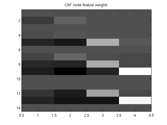
We will solve min_{w,v} nll(w,v,x,y) + lambda * sum_f |w_f|_2, where nll(w,v,x,y) is the negative log-likelihood for a log-linear chain-structured conditional random field and each 'group' f is the set of parameters associated with a single input feature, leading to sparsity in the terms of the input features
load wordData.mat
lambda = 20;

% Initialize
[w,vs,ve,v] = crfChain_initWeights(nFeatures,nStates);
featureStart = cumsum([1 nFeatures(1:end)]); % data structure which relates high-level 'features' to elements of w
sentences = crfChain_initSentences(y);
nSentences = size(sentences,1);
maxSentenceLength = 1+max(sentences(:,2)-sentences(:,1));
wv = [w(:);vs;ve;v(:)];
nVars = length(wv);
funObj = @(wv)crfChain_loss(wv,X,y,nStates,nFeatures,featureStart,sentences);

% Put all node variables associated with individual features into groups
groups_w = repmat([1:sum(nFeatures)]',[1 nStates]);

% Don't penalize edge variables
groups_vs= zeros(size(vs));
groups_ve= zeros(size(ve));
groups_v= zeros(size(v));

groups = [groups_w(:);groups_vs;groups_ve;groups_v(:)];
nGroups = max(groups);

% Initialize auxiliary variables
alpha = zeros(nGroups,1);
penalizedFunObj = @(w)auxGroupLoss(w,groups,lambda,funObj);

% Set up L_1,2 Projection Function
[groupStart,groupPtr] = groupl1_makeGroupPointers(groups);
funProj = @(w)auxGroupL2Project(w,nVars,groupStart,groupPtr);

% Solve with PQN
fprintf('\nComputing feature-sparse conditional random field parameters...\n');
wva = minConf_PQN(penalizedFunObj,[wv;alpha],funProj);

[w,vs,ve,v] = crfChain_splitWeights(wva(1:nVars),featureStart,nStates);

figure
imagesc(w);colormap gray
title('CRF node feature weights');
pause
Computing feature-sparse conditional random field parameters...
 Iteration   FunEvals Projections     Step Length    Function Val        Opt Cond
         1          2          4     4.13907e-04     1.16766e+03     6.31389e+01
         2          3         16     1.00000e+00     8.79023e+02     5.35717e+01
         3          4         28     1.00000e+00     8.39557e+02     2.54508e+01
         4          5         40     1.00000e+00     8.20969e+02     1.41169e+01
         5          6         51     1.00000e+00     7.96231e+02     1.32832e+01
         6          7         63     1.00000e+00     7.78225e+02     6.46104e+00
         7          8         75     1.00000e+00     7.72086e+02     3.19869e+00
         8          9         87     1.00000e+00     7.67519e+02     1.11609e+01
         9         10         99     1.00000e+00     7.64916e+02     5.39515e+00
        10         11        111     1.00000e+00     7.61398e+02     5.54300e+00
        11         12        123     1.00000e+00     7.59558e+02     4.14841e+00
        12         13        135     1.00000e+00     7.58421e+02     1.17329e+00
        13         14        147     1.00000e+00     7.58089e+02     2.69375e+00
        14         15        158     1.00000e+00     7.57927e+02     2.16008e+00
        15         16        170     1.00000e+00     7.57711e+02     8.79680e-01
        16         17        182     1.00000e+00     7.57668e+02     4.16621e-01
        17         18        194     1.00000e+00     7.57648e+02     2.19777e-01
        18         19        206     1.00000e+00     7.57641e+02     1.48976e-01
        19         20        218     1.00000e+00     7.57639e+02     1.41745e-01
        20         21        230     1.00000e+00     7.57637e+02     1.02384e-01
        21         22        242     1.00000e+00     7.57636e+02     5.13171e-02
        22         23        253     1.00000e+00     7.57636e+02     3.34465e-02
        23         24        265     1.00000e+00     7.57636e+02     1.65591e-02
        24         25        277     1.00000e+00     7.57636e+02     1.18514e-02
        25         26        289     1.00000e+00     7.57636e+02     7.18780e-03
        26         27        301     1.00000e+00     7.57636e+02     4.87103e-03
        27         28        313     1.00000e+00     7.57636e+02     3.04077e-03
        28         29        325     1.00000e+00     7.57636e+02     2.40636e-03
        29         30        337     1.00000e+00     7.57636e+02     1.00814e-03
        30         31        348     1.00000e+00     7.57636e+02     5.67028e-04
        31         32        360     1.00000e+00     7.57636e+02     5.51060e-04
        32         33        370     1.00000e+00     7.57636e+02     3.93047e-04
        33         34        381     1.00000e+00     7.57636e+02     2.28419e-04
        34         35        393     1.00000e+00     7.57636e+02     1.40384e-04
        35         36        398     1.00000e+00     7.57636e+02     1.49688e-04
Function value changing by less than progTol
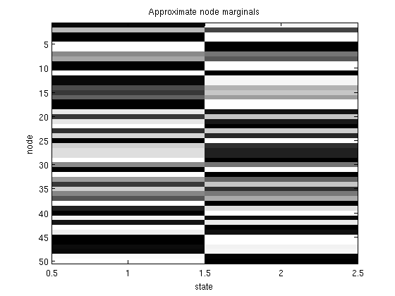
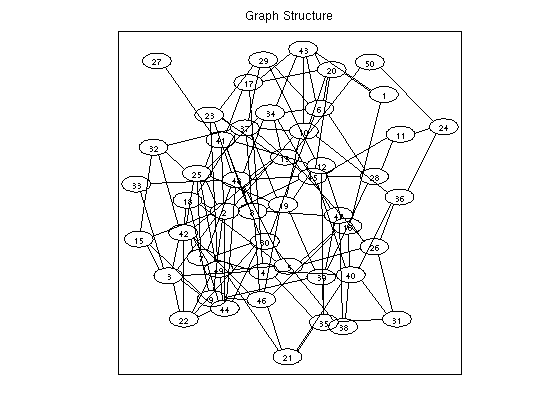
Approximating node marginals in undirected graphical models with variational mean field
We want to approximate marginals in a pairwise Markov random field by minimizing the Gibbs free energy under a mean-field (factorized) approximation.
Variational approximations and the mean field free energy are described in: Yedidia, Freeman, Weiss. Understanding Belief Propagation and Its Generalizations. IJCAI (2001).
The projection reduces to a series of independent projections on the simplex.
% Generate potentials a pairiwse graphical model
nNodes = 50;
nStates = 2;
adj = zeros(nNodes);
for n1 = 1:nNodes
    for n2 = n1+1:nNodes
        if rand > .9
           adj(n1,n2) = 1;
           adj(n2,n1) = 1;
        end
    end
end
edgeStruct = UGM_makeEdgeStruct(adj,nStates);
nEdges = edgeStruct.nEdges;
edgeEnds = edgeStruct.edgeEnds;
nodePot = rand(nNodes,nStates);
edgePot = rand(nStates,nStates,nEdges);

% Intialize marginals
nodeBel = (1/nStates)*ones(nNodes,nStates);

% Make objective function
funObj = @(nodeBel)MeanFieldGibbsFreeEnergyLoss(nodeBel,nodePot,edgePot,edgeEnds);

% Make projection function
funProj = @(nodeBel)MeanFieldGibbsFreeEnergyProject(nodeBel,nNodes,nStates);

% Solve with PQN
fprintf('\nMinimizing Mean Field Gibbs Free Energy of pairwise undirected graphical model...\n');
nodeBel(:) = minConf_PQN(funObj,nodeBel(:),funProj);

figure
imagesc(nodeBel);colormap gray
title('Approximate node marginals');
ylabel('node');
xlabel('state');
figure
drawGraph(adj);
title('Graph Structure');
pause
Minimizing Mean Field Gibbs Free Energy of pairwise undirected graphical model...
 Iteration   FunEvals Projections     Step Length    Function Val        Opt Cond
         1          2          4     1.44167e-03     1.62658e+02     4.99279e-01
         2          3         16     1.00000e+00     1.31962e+02     8.52303e-01
         3          4         28     1.00000e+00     1.30132e+02     7.80049e-01
         4          5         40     1.00000e+00     1.27262e+02     4.72673e-01
         5          6         52     1.00000e+00     1.26291e+02     4.18405e-01
         6          7         64     1.00000e+00     1.26151e+02     4.03896e-01
         7          8         76     1.00000e+00     1.25875e+02     9.99358e-01
         8          9         88     1.00000e+00     1.25780e+02     3.45929e-01
         9         10         99     1.00000e+00     1.25711e+02     3.52333e-01
        10         11        109     1.00000e+00     1.25578e+02     3.97842e-01
        11         12        120     1.00000e+00     1.25422e+02     5.79143e-01
        12         13        131     1.00000e+00     1.25320e+02     2.18241e-01
        13         14        142     1.00000e+00     1.25227e+02     2.20488e-01
        14         15        153     1.00000e+00     1.25136e+02     2.40032e-01
        15         16        164     1.00000e+00     1.25029e+02     2.13415e-01
        16         17        175     1.00000e+00     1.24977e+02     1.80182e-01
        17         18        186     1.00000e+00     1.24944e+02     3.82755e-01
        18         19        198     1.00000e+00     1.24935e+02     3.28613e-01
        19         20        210     1.00000e+00     1.24927e+02     1.29281e-01
        20         21        221     1.00000e+00     1.24919e+02     1.89010e-01
        21         22        233     1.00000e+00     1.24916e+02     5.97267e-02
        22         23        245     1.00000e+00     1.24914e+02     4.86406e-02
        23         24        256     1.00000e+00     1.24912e+02     3.25016e-02
        24         25        267     1.00000e+00     1.24911e+02     2.93020e-02
        25         26        278     1.00000e+00     1.24911e+02     2.23381e-02
        26         27        289     1.00000e+00     1.24910e+02     2.25549e-02
        27         28        301     1.00000e+00     1.24910e+02     1.32620e-02
        28         29        313     1.00000e+00     1.24910e+02     1.36705e-02
        29         30        325     1.00000e+00     1.24910e+02     9.27483e-03
        30         31        337     1.00000e+00     1.24910e+02     5.73696e-03
        31         32        349     1.00000e+00     1.24910e+02     3.15075e-03
        32         33        360     1.00000e+00     1.24910e+02     3.61176e-03
        33         34        372     1.00000e+00     1.24910e+02     2.62249e-03
        34         35        383     1.00000e+00     1.24910e+02     1.14729e-03
        35         36        395     1.00000e+00     1.24910e+02     1.92095e-03
        36         37        406     1.00000e+00     1.24910e+02     1.02304e-03
        37         38        418     1.00000e+00     1.24910e+02     7.10496e-04
        38         39        429     1.00000e+00     1.24910e+02     4.60186e-04
        39         40        441     1.00000e+00     1.24910e+02     2.55750e-04
        40         41        452     1.00000e+00     1.24910e+02     1.81987e-04
        41         42        463     1.00000e+00     1.24910e+02     1.66579e-04
        42         43        474     1.00000e+00     1.24910e+02     3.50226e-04
        43         44        484     1.00000e+00     1.24910e+02     1.58874e-04
        44         45        496     1.00000e+00     1.24910e+02     3.99517e-05
Directional Derivative below progTol
neato - Graphviz version 2.20.2 (Tue Mar  2 19:03:41 UTC 2010)
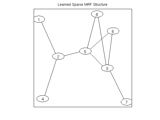
Multi-State Markov Random Field Structure Learning
We will solve min_{w,v} nll(w,v,y), s.t. sum_e |v_e|_2 <= tau, where nll(w,v,y) is the negative log-likelihood for a log-linear Markov random field and each 'group' e is the set of parameters associated with an edge, leading to sparsity in the graph
Using group-sparsity to select edges in a multi-state Markov random field is discussed in: Schmidt, Murphy, Fung, and Rosales. Structure Learning in Random Field for Heart Motion Abnormality Detection. CVPR (2008).
% Generate Data
nInstances = 250;
nNodes = 8;
edgeDensity = .33;
nStates = 3;
ising = 0;
tied = 0;
useMex = 1;
y = UGM_generate(nInstances,0,nNodes,edgeDensity,nStates,ising,tied);

% Set up MRF
adj = fullAdjMatrix(nNodes);
edgeStruct = UGM_makeEdgeStruct(adj,nStates,useMex);
[nodeMap,edgeMap] = UGM_makeMRFmaps(edgeStruct,ising,tied);

% Initialize Variables
nNodeParams = max(nodeMap(:));
nParams = max(edgeMap(:));
nEdgeParams = nParams-nNodeParams;
w = zeros(nParams,1);

% Make Groups
groups = zeros(nParams,1);
for e = 1:edgeStruct.nEdges
	edgeParams = edgeMap(:,:,e,:);
	groups(edgeParams(:)) = e;
end

% Set up Objective Function
suffStat = UGM_MRF_computeSuffStat(y,nodeMap,edgeMap,edgeStruct);
funObj = @(w)UGM_MRF_NLL(w,nInstances,suffStat,nodeMap,edgeMap,edgeStruct,@UGM_Infer_Exact);
lambdaL2 = 1;
penalizedFunObj = @(w)penalizedL2(w,funObj,lambdaL2);

% Set up L_1,2 Projection Function
tau = 5;
funProj = @(w)groupL2Proj(w,tau,groups);

% Solve with PQN
fprintf('\nComputing Sparse Markov random field parameters...\n');
w = minConf_PQN(penalizedFunObj,w,funProj);
w(abs(w) < 1e-4) = 0;

% Check selected variables
for e = 1:edgeStruct.nEdges
	params = edgeMap(:,:,e);
	params = params(params(:)~=0);
   fprintf('Number of non-zero variables associated with edge from %d to %d: %d (of %d)\n',edgeStruct.edgeEnds(e,1),edgeStruct.edgeEnds(e,2),nnz(w(params)),numel(w(params)));
end

% Make final adjacency matrix
adj = zeros(nNodes);
for e = 1:edgeStruct.nEdges
	params = edgeMap(:,:,e);
	params = params(params(:)~=0);
    if any(w(params)~=0)
        n1 = edgeStruct.edgeEnds(e,1);
        n2 = edgeStruct.edgeEnds(e,2);
        adj(n1,n2) = 1;
        adj(n2,n1) = 1;
    end
end
figure
drawGraph(adj);
title('Learned Sparse MRF Structure');
pause
Exact Sampling

Computing Sparse Markov random field parameters...
 Iteration   FunEvals Projections     Step Length    Function Val        Opt Cond
         1          2          4     8.65202e-05     2.18482e+03     1.61649e+02
         2          3         16     1.00000e+00     8.58677e+02     1.98063e+01
         3          4         28     1.00000e+00     8.39193e+02     1.27737e+01
         4          5         40     1.00000e+00     8.27884e+02     9.19846e+00
         5          6         52     1.00000e+00     8.11888e+02     4.33189e+00
         6          7         63     1.00000e+00     8.11244e+02     2.39436e+01
         7          8         75     1.00000e+00     8.05800e+02     6.99203e+00
         8          9         87     1.00000e+00     8.04591e+02     3.73055e+00
         9         10         99     1.00000e+00     8.03432e+02     4.10645e+00
        10         11        111     1.00000e+00     8.02194e+02     4.28152e+00
        11         12        123     1.00000e+00     8.01689e+02     7.51540e+00
        12         13        135     1.00000e+00     8.01154e+02     3.91117e+00
        13         14        147     1.00000e+00     8.00701e+02     3.32273e+00
        14         15        158     1.00000e+00     8.00312e+02     2.69325e+00
        15         16        168     1.00000e+00     7.99896e+02     2.15604e+00
        16         17        179     1.00000e+00     7.99403e+02     2.38568e+00
        17         18        190     1.00000e+00     7.98913e+02     2.16397e+00
        18         19        201     1.00000e+00     7.98279e+02     1.17471e+00
        19         20        212     1.00000e+00     7.97936e+02     7.70176e-01
        20         21        224     1.00000e+00     7.97840e+02     7.30143e-01
        21         22        235     1.00000e+00     7.97762e+02     7.60268e-01
        22         23        246     1.00000e+00     7.97702e+02     5.70059e-01
        23         24        257     1.00000e+00     7.97658e+02     1.41639e+00
        24         25        269     1.00000e+00     7.97633e+02     5.35854e-01
        25         26        281     1.00000e+00     7.97622e+02     4.00744e-01
        26         27        292     1.00000e+00     7.97608e+02     3.74958e-01
        27         28        303     1.00000e+00     7.97593e+02     3.44633e-01
        28         29        314     1.00000e+00     7.97571e+02     2.65858e-01
        29         30        325     1.00000e+00     7.97554e+02     2.33143e-01
        30         31        336     1.00000e+00     7.97532e+02     1.99139e-01
        31         32        348     1.00000e+00     7.97528e+02     1.45973e-01
        32         33        359     1.00000e+00     7.97525e+02     1.30455e-01
        33         34        370     1.00000e+00     7.97523e+02     7.77846e-02
        34         35        381     1.00000e+00     7.97522e+02     1.20532e-01
        35         36        392     1.00000e+00     7.97522e+02     1.04226e-01
        36         37        403     1.00000e+00     7.97521e+02     4.47146e-02
        37         38        414     1.00000e+00     7.97521e+02     4.32276e-02
        38         39        425     1.00000e+00     7.97520e+02     3.88135e-02
        39         40        436     1.00000e+00     7.97520e+02     3.51474e-02
        40         41        447     1.00000e+00     7.97520e+02     2.60144e-02
        41         42        459     1.00000e+00     7.97520e+02     3.59869e-02
        42         43        471     1.00000e+00     7.97520e+02     2.77704e-02
        43         44        481     1.00000e+00     7.97520e+02     1.61027e-02
        44         45        493     1.00000e+00     7.97519e+02     1.43819e-02
        45         46        504     1.00000e+00     7.97519e+02     1.31595e-02
        46         47        515     1.00000e+00     7.97519e+02     1.10195e-02
        47         48        527     1.00000e+00     7.97519e+02     8.98387e-03
        48         49        538     1.00000e+00     7.97519e+02     5.68701e-03
        49         50        550     1.00000e+00     7.97519e+02     5.86993e-03
        50         51        562     1.00000e+00     7.97519e+02     4.57134e-03
        51         52        574     1.00000e+00     7.97519e+02     2.45114e-03
        52         53        586     1.00000e+00     7.97519e+02     1.90106e-03
        53         54        598     1.00000e+00     7.97519e+02     2.00244e-03
        54         55        610     1.00000e+00     7.97519e+02     1.07678e-03
        55         56        622     1.00000e+00     7.97519e+02     6.61842e-04
        56         57        634     1.00000e+00     7.97519e+02     7.38063e-04
        57         58        646     1.00000e+00     7.97519e+02     7.70531e-04
        58         59        657     1.00000e+00     7.97519e+02     5.81262e-04
        59         60        668     1.00000e+00     7.97519e+02     4.27253e-04
        60         61        680     1.00000e+00     7.97519e+02     9.88395e-04
        61         62        692     1.00000e+00     7.97519e+02     5.59799e-04
        62         63        703     1.00000e+00     7.97519e+02     4.07185e-04
        63         64        714     1.00000e+00     7.97519e+02     3.34542e-04
        64         65        725     1.00000e+00     7.97519e+02     3.45916e-04
        65         66        736     1.00000e+00     7.97519e+02     2.90131e-04
        66         67        747     1.00000e+00     7.97519e+02     2.41294e-04
        67         68        758     1.00000e+00     7.97519e+02     1.68164e-04
        68         69        769     1.00000e+00     7.97519e+02     1.21657e-04
        69         70        776     1.00000e+00     7.97519e+02     1.26649e-04
Directional Derivative below progTol
Number of non-zero variables associated with edge from 1 to 2: 9 (of 9)
Number of non-zero variables associated with edge from 1 to 3: 0 (of 9)
Number of non-zero variables associated with edge from 1 to 4: 0 (of 9)
Number of non-zero variables associated with edge from 1 to 5: 0 (of 9)
Number of non-zero variables associated with edge from 1 to 6: 0 (of 9)
Number of non-zero variables associated with edge from 1 to 7: 0 (of 9)
Number of non-zero variables associated with edge from 1 to 8: 0 (of 9)
Number of non-zero variables associated with edge from 2 to 3: 0 (of 9)
Number of non-zero variables associated with edge from 2 to 4: 9 (of 9)
Number of non-zero variables associated with edge from 2 to 5: 9 (of 9)
Number of non-zero variables associated with edge from 2 to 6: 0 (of 9)
Number of non-zero variables associated with edge from 2 to 7: 0 (of 9)
Number of non-zero variables associated with edge from 2 to 8: 0 (of 9)
Number of non-zero variables associated with edge from 3 to 4: 0 (of 9)
Number of non-zero variables associated with edge from 3 to 5: 9 (of 9)
Number of non-zero variables associated with edge from 3 to 6: 9 (of 9)
Number of non-zero variables associated with edge from 3 to 7: 9 (of 9)
Number of non-zero variables associated with edge from 3 to 8: 9 (of 9)
Number of non-zero variables associated with edge from 4 to 5: 0 (of 9)
Number of non-zero variables associated with edge from 4 to 6: 0 (of 9)
Number of non-zero variables associated with edge from 4 to 7: 0 (of 9)
Number of non-zero variables associated with edge from 4 to 8: 0 (of 9)
Number of non-zero variables associated with edge from 5 to 6: 9 (of 9)
Number of non-zero variables associated with edge from 5 to 7: 0 (of 9)
Number of non-zero variables associated with edge from 5 to 8: 9 (of 9)
Number of non-zero variables associated with edge from 6 to 7: 0 (of 9)
Number of non-zero variables associated with edge from 6 to 8: 0 (of 9)
Number of non-zero variables associated with edge from 7 to 8: 0 (of 9)
neato - Graphviz version 2.20.2 (Tue Mar  2 19:03:41 UTC 2010)
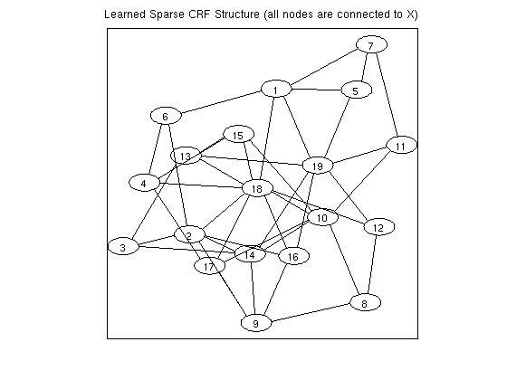
Conditional Random Field Structure Learning with Pseudo-Likelihood
We will solve min_{w,v} nll(w,v,x,y) + lambda * sum_e |v_e|_inf, where nll(w,v,x,y) is the negative log-likelihood for a log-linear conditional random field and each 'group' e is the set of parameters associated with an edge, leading to sparsity in the graph
To solve the problem, we use a pseudo-likelihood approximation of the negative log-likelihood, and convert the non-differentiable problem to a differentiable one by introducing auxiliary variables
Using group-sparsity to select edges in a conditional random field trained with pseudo-likelihood is discussed in: Schmidt, Murphy, Fung, and Rosales. Structure Learning in Random Field for Heart Motion Abnormality Detection. CVPR (2008).
% Generate Data
nInstances = 250;
nFeatures = 10;
nNodes = 20;
edgeDensity = .25;
nStates = 2;
ising = 0;
tied = 0;
useMex = 1;
[y,adj,X] = UGM_generate(nInstances,nFeatures,nNodes,edgeDensity,nStates,ising,tied);

% Set up CRF
adj = fullAdjMatrix(nNodes);
edgeStruct = UGM_makeEdgeStruct(adj,nStates,useMex);

% Make edge features
Xedge = UGM_makeEdgeFeatures(X,edgeStruct.edgeEnds);
[nodeMap,edgeMap] = UGM_makeCRFmaps(X,Xedge,edgeStruct,ising,tied);

% Initialize Variables
nNodeParams = max(nodeMap(:));
nVars = max(edgeMap(:));
w = zeros(nVars,1);

% Make Groups
groups = zeros(nVars,1);
for e = 1:edgeStruct.nEdges
	edgeParams = edgeMap(:,:,e,:);
	groups(edgeParams(:)) = e;
end
nGroups = edgeStruct.nEdges;

% Set up Objective Function
funObj = @(w)UGM_CRF_PseudoNLL(w,X,Xedge,y,nodeMap,edgeMap,edgeStruct);
lambdaL2 = 1;
penalizedFunObj = @(w)penalizedL2(w,funObj,lambdaL2);

% Initialize auxiliary variables that will bound norm
lambda = 500;
alpha = zeros(nGroups,1);
auxFunObj = @(wAlpha)auxGroupLoss(wAlpha,groups,lambda,penalizedFunObj);

% Set up L_1,inf Projection Function
[groupStart,groupPtr] = groupl1_makeGroupPointers(groups);
funProj = @(wAlpha)auxGroupLinfProject(wAlpha,nVars,groupStart,groupPtr);

% Solve with PQN
fprintf('\nComputing Sparse conditional random field parameters...\n');
wAlpha = minConf_PQN(auxFunObj,[w;alpha],funProj);
w = wAlpha(1:nVars);
w(abs(w) < 1e-4) = 0;

% Check selected variables
for e = 1:edgeStruct.nEdges
	params = edgeMap(:,:,e,:);
	params = params(params(:)~=0);
   fprintf('Number of non-zero variables associated with edge from %d to %d: %d (of %d)\n',edgeStruct.edgeEnds(e,1),edgeStruct.edgeEnds(e,2),nnz(w(params)),numel(w(params)));
end

% Make final adjacency matrix
adj = zeros(nNodes);
for e = 1:edgeStruct.nEdges
	params = edgeMap(:,:,e,:);
	params = params(params(:)~=0);
    if any(w(params)~=0)
        n1 = edgeStruct.edgeEnds(e,1);
        n2 = edgeStruct.edgeEnds(e,2);
        adj(n1,n2) = 1;
        adj(n2,n1) = 1;
    end
end
figure
drawGraph(adj);
title('Learned Sparse CRF Structure (all nodes are connected to X)');
Gibbs Sampling

Computing Sparse conditional random field parameters...
 Iteration   FunEvals Projections     Step Length    Function Val        Opt Cond
         1          2          4     3.52789e-06     3.46298e+03     6.37126e+01
         2          3         16     1.00000e+00     2.96765e+03     3.31060e+01
         3          4         28     1.00000e+00     2.88935e+03     2.62199e+01
         4          5         39     1.00000e+00     2.76144e+03     1.65791e+01
         5          6         50     1.00000e+00     2.65383e+03     1.21515e+01
         6          7         61     1.00000e+00     2.56483e+03     1.07178e+01
         7          8         73     1.00000e+00     2.51620e+03     8.46672e+00
         8          9         85     1.00000e+00     2.48459e+03     5.90253e+00
         9         10         97     1.00000e+00     2.46736e+03     4.42851e+00
        10         11        109     1.00000e+00     2.45945e+03     3.27385e+00
        11         12        121     1.00000e+00     2.45521e+03     2.24937e+00
        12         13        133     1.00000e+00     2.45361e+03     1.65477e+00
        13         14        145     1.00000e+00     2.45242e+03     1.17876e+00
        14         15        157     1.00000e+00     2.45191e+03     9.55383e-01
        15         16        169     1.00000e+00     2.45156e+03     6.70175e-01
        16         17        181     1.00000e+00     2.45138e+03     5.36553e-01
        17         18        193     1.00000e+00     2.45128e+03     4.16853e-01
        18         19        205     1.00000e+00     2.45123e+03     3.04263e-01
        19         20        217     1.00000e+00     2.45120e+03     2.06939e-01
        20         21        229     1.00000e+00     2.45119e+03     1.39867e-01
        21         22        241     1.00000e+00     2.45118e+03     1.03235e-01
        22         23        253     1.00000e+00     2.45117e+03     7.68651e-02
        23         24        265     1.00000e+00     2.45117e+03     5.60913e-02
        24         25        277     1.00000e+00     2.45117e+03     4.48514e-02
        25         26        289     1.00000e+00     2.45117e+03     4.21212e-02
        26         27        301     1.00000e+00     2.45116e+03     2.97279e-02
        27         28        313     1.00000e+00     2.45116e+03     3.80838e-02
        28         29        324     1.00000e+00     2.45116e+03     4.14760e-02
        29         30        335     1.00000e+00     2.45116e+03     4.08802e-02
        30         31        347     1.00000e+00     2.45116e+03     2.81035e-02
        31         32        358     1.00000e+00     2.45116e+03     3.07415e-02
        32         33        369     1.00000e+00     2.45116e+03     3.11472e-02
        33         34        380     1.00000e+00     2.45116e+03     3.06254e-02
        34         35        391     1.00000e+00     2.45116e+03     3.77315e-02
        35         36        403     1.00000e+00     2.45116e+03     4.23843e-02
        36         37        415     1.00000e+00     2.45116e+03     3.87756e-02
        37         38        427     1.00000e+00     2.45116e+03     3.13473e-02
        38         39        438     1.00000e+00     2.45116e+03     2.59070e-02
        39         40        450     1.00000e+00     2.45116e+03     2.61268e-02
        40         41        462     1.00000e+00     2.45116e+03     2.27940e-02
        41         42        474     1.00000e+00     2.45116e+03     1.81264e-02
        42         43        485     1.00000e+00     2.45116e+03     1.52857e-02
        43         44        496     1.00000e+00     2.45116e+03     1.76452e-02
        44         45        508     1.00000e+00     2.45116e+03     2.07862e-02
        45         46        518     1.00000e+00     2.45116e+03     1.75046e-02
        46         47        529     1.00000e+00     2.45116e+03     1.41643e-02
        47         48        540     1.00000e+00     2.45116e+03     1.38166e-02
        48         49        550     1.00000e+00     2.45116e+03     1.26736e-02
        49         50        561     1.00000e+00     2.45116e+03     1.00676e-02
        50         51        572     1.00000e+00     2.45116e+03     9.68540e-03
        51         52        584     1.00000e+00     2.45116e+03     9.93275e-03
        52         53        595     1.00000e+00     2.45116e+03     9.95888e-03
        53         54        606     1.00000e+00     2.45116e+03     8.51003e-03
        54         55        617     1.00000e+00     2.45116e+03     9.56613e-03
        55         56        628     1.00000e+00     2.45116e+03     1.14717e-02
        56         57        640     1.00000e+00     2.45116e+03     1.10797e-02
        57         58        652     1.00000e+00     2.45116e+03     9.66020e-03
        58         59        664     1.00000e+00     2.45116e+03     7.12239e-03
        59         60        675     1.00000e+00     2.45116e+03     9.70268e-03
        60         61        686     1.00000e+00     2.45116e+03     1.06271e-02
        61         62        697     1.00000e+00     2.45116e+03     8.66663e-03
        62         63        709     1.00000e+00     2.45116e+03     5.21659e-03
        63         64        720     1.00000e+00     2.45116e+03     8.04831e-03
        64         65        732     1.00000e+00     2.45116e+03     6.38215e-03
        65         66        743     1.00000e+00     2.45116e+03     7.36685e-03
        66         67        755     1.00000e+00     2.45116e+03     9.52317e-03
        67         68        766     1.00000e+00     2.45116e+03     7.16611e-03
        68         69        777     1.00000e+00     2.45116e+03     5.36047e-03
        69         70        788     1.00000e+00     2.45116e+03     5.32784e-03
        70         71        800     1.00000e+00     2.45116e+03     4.36776e-03
        71         72        812     1.00000e+00     2.45116e+03     3.60682e-03
        72         73        823     1.00000e+00     2.45116e+03     2.98529e-03
        73         74        834     1.00000e+00     2.45116e+03     3.28175e-03
        74         75        846     1.00000e+00     2.45116e+03     3.00937e-03
        75         76        858     1.00000e+00     2.45116e+03     3.05478e-03
        76         77        870     1.00000e+00     2.45116e+03     2.93148e-03
        77         78        882     1.00000e+00     2.45116e+03     2.35747e-03
        78         79        893     1.00000e+00     2.45116e+03     2.20906e-03
        79         80        904     1.00000e+00     2.45116e+03     2.15725e-03
        80         81        916     1.00000e+00     2.45116e+03     1.69084e-03
        81         82        928     1.00000e+00     2.45116e+03     1.66883e-03
        82         83        940     1.00000e+00     2.45116e+03     1.43711e-03
Directional Derivative below progTol
Number of non-zero variables associated with edge from 1 to 2: 0 (of 80)
Number of non-zero variables associated with edge from 1 to 3: 0 (of 80)
Number of non-zero variables associated with edge from 1 to 4: 0 (of 80)
Number of non-zero variables associated with edge from 1 to 5: 80 (of 80)
Number of non-zero variables associated with edge from 1 to 6: 80 (of 80)
Number of non-zero variables associated with edge from 1 to 7: 80 (of 80)
Number of non-zero variables associated with edge from 1 to 8: 0 (of 80)
Number of non-zero variables associated with edge from 1 to 9: 0 (of 80)
Number of non-zero variables associated with edge from 1 to 10: 0 (of 80)
Number of non-zero variables associated with edge from 1 to 11: 0 (of 80)
Number of non-zero variables associated with edge from 1 to 12: 0 (of 80)
Number of non-zero variables associated with edge from 1 to 13: 0 (of 80)
Number of non-zero variables associated with edge from 1 to 14: 0 (of 80)
Number of non-zero variables associated with edge from 1 to 15: 0 (of 80)
Number of non-zero variables associated with edge from 1 to 16: 0 (of 80)
Number of non-zero variables associated with edge from 1 to 17: 0 (of 80)
Number of non-zero variables associated with edge from 1 to 18: 80 (of 80)
Number of non-zero variables associated with edge from 1 to 19: 80 (of 80)
Number of non-zero variables associated with edge from 1 to 20: 0 (of 80)
Number of non-zero variables associated with edge from 2 to 3: 80 (of 80)
Number of non-zero variables associated with edge from 2 to 4: 0 (of 80)
Number of non-zero variables associated with edge from 2 to 5: 0 (of 80)
Number of non-zero variables associated with edge from 2 to 6: 80 (of 80)
Number of non-zero variables associated with edge from 2 to 7: 0 (of 80)
Number of non-zero variables associated with edge from 2 to 8: 0 (of 80)
Number of non-zero variables associated with edge from 2 to 9: 80 (of 80)
Number of non-zero variables associated with edge from 2 to 10: 0 (of 80)
Number of non-zero variables associated with edge from 2 to 11: 0 (of 80)
Number of non-zero variables associated with edge from 2 to 12: 0 (of 80)
Number of non-zero variables associated with edge from 2 to 13: 0 (of 80)
Number of non-zero variables associated with edge from 2 to 14: 80 (of 80)
Number of non-zero variables associated with edge from 2 to 15: 0 (of 80)
Number of non-zero variables associated with edge from 2 to 16: 80 (of 80)
Number of non-zero variables associated with edge from 2 to 17: 0 (of 80)
Number of non-zero variables associated with edge from 2 to 18: 80 (of 80)
Number of non-zero variables associated with edge from 2 to 19: 0 (of 80)
Number of non-zero variables associated with edge from 2 to 20: 0 (of 80)
Number of non-zero variables associated with edge from 3 to 4: 0 (of 80)
Number of non-zero variables associated with edge from 3 to 5: 0 (of 80)
Number of non-zero variables associated with edge from 3 to 6: 0 (of 80)
Number of non-zero variables associated with edge from 3 to 7: 0 (of 80)
Number of non-zero variables associated with edge from 3 to 8: 0 (of 80)
Number of non-zero variables associated with edge from 3 to 9: 0 (of 80)
Number of non-zero variables associated with edge from 3 to 10: 0 (of 80)
Number of non-zero variables associated with edge from 3 to 11: 0 (of 80)
Number of non-zero variables associated with edge from 3 to 12: 0 (of 80)
Number of non-zero variables associated with edge from 3 to 13: 80 (of 80)
Number of non-zero variables associated with edge from 3 to 14: 80 (of 80)
Number of non-zero variables associated with edge from 3 to 15: 0 (of 80)
Number of non-zero variables associated with edge from 3 to 16: 0 (of 80)
Number of non-zero variables associated with edge from 3 to 17: 0 (of 80)
Number of non-zero variables associated with edge from 3 to 18: 0 (of 80)
Number of non-zero variables associated with edge from 3 to 19: 0 (of 80)
Number of non-zero variables associated with edge from 3 to 20: 0 (of 80)
Number of non-zero variables associated with edge from 4 to 5: 0 (of 80)
Number of non-zero variables associated with edge from 4 to 6: 80 (of 80)
Number of non-zero variables associated with edge from 4 to 7: 0 (of 80)
Number of non-zero variables associated with edge from 4 to 8: 0 (of 80)
Number of non-zero variables associated with edge from 4 to 9: 0 (of 80)
Number of non-zero variables associated with edge from 4 to 10: 0 (of 80)
Number of non-zero variables associated with edge from 4 to 11: 0 (of 80)
Number of non-zero variables associated with edge from 4 to 12: 0 (of 80)
Number of non-zero variables associated with edge from 4 to 13: 0 (of 80)
Number of non-zero variables associated with edge from 4 to 14: 0 (of 80)
Number of non-zero variables associated with edge from 4 to 15: 80 (of 80)
Number of non-zero variables associated with edge from 4 to 16: 0 (of 80)
Number of non-zero variables associated with edge from 4 to 17: 80 (of 80)
Number of non-zero variables associated with edge from 4 to 18: 80 (of 80)
Number of non-zero variables associated with edge from 4 to 19: 0 (of 80)
Number of non-zero variables associated with edge from 4 to 20: 0 (of 80)
Number of non-zero variables associated with edge from 5 to 6: 0 (of 80)
Number of non-zero variables associated with edge from 5 to 7: 80 (of 80)
Number of non-zero variables associated with edge from 5 to 8: 0 (of 80)
Number of non-zero variables associated with edge from 5 to 9: 0 (of 80)
Number of non-zero variables associated with edge from 5 to 10: 0 (of 80)
Number of non-zero variables associated with edge from 5 to 11: 0 (of 80)
Number of non-zero variables associated with edge from 5 to 12: 0 (of 80)
Number of non-zero variables associated with edge from 5 to 13: 0 (of 80)
Number of non-zero variables associated with edge from 5 to 14: 0 (of 80)
Number of non-zero variables associated with edge from 5 to 15: 0 (of 80)
Number of non-zero variables associated with edge from 5 to 16: 0 (of 80)
Number of non-zero variables associated with edge from 5 to 17: 0 (of 80)
Number of non-zero variables associated with edge from 5 to 18: 0 (of 80)
Number of non-zero variables associated with edge from 5 to 19: 80 (of 80)
Number of non-zero variables associated with edge from 5 to 20: 0 (of 80)
Number of non-zero variables associated with edge from 6 to 7: 0 (of 80)
Number of non-zero variables associated with edge from 6 to 8: 0 (of 80)
Number of non-zero variables associated with edge from 6 to 9: 0 (of 80)
Number of non-zero variables associated with edge from 6 to 10: 0 (of 80)
Number of non-zero variables associated with edge from 6 to 11: 0 (of 80)
Number of non-zero variables associated with edge from 6 to 12: 0 (of 80)
Number of non-zero variables associated with edge from 6 to 13: 0 (of 80)
Number of non-zero variables associated with edge from 6 to 14: 0 (of 80)
Number of non-zero variables associated with edge from 6 to 15: 0 (of 80)
Number of non-zero variables associated with edge from 6 to 16: 0 (of 80)
Number of non-zero variables associated with edge from 6 to 17: 0 (of 80)
Number of non-zero variables associated with edge from 6 to 18: 0 (of 80)
Number of non-zero variables associated with edge from 6 to 19: 0 (of 80)
Number of non-zero variables associated with edge from 6 to 20: 0 (of 80)
Number of non-zero variables associated with edge from 7 to 8: 0 (of 80)
Number of non-zero variables associated with edge from 7 to 9: 0 (of 80)
Number of non-zero variables associated with edge from 7 to 10: 0 (of 80)
Number of non-zero variables associated with edge from 7 to 11: 80 (of 80)
Number of non-zero variables associated with edge from 7 to 12: 0 (of 80)
Number of non-zero variables associated with edge from 7 to 13: 0 (of 80)
Number of non-zero variables associated with edge from 7 to 14: 0 (of 80)
Number of non-zero variables associated with edge from 7 to 15: 0 (of 80)
Number of non-zero variables associated with edge from 7 to 16: 0 (of 80)
Number of non-zero variables associated with edge from 7 to 17: 0 (of 80)
Number of non-zero variables associated with edge from 7 to 18: 0 (of 80)
Number of non-zero variables associated with edge from 7 to 19: 0 (of 80)
Number of non-zero variables associated with edge from 7 to 20: 0 (of 80)
Number of non-zero variables associated with edge from 8 to 9: 80 (of 80)
Number of non-zero variables associated with edge from 8 to 10: 80 (of 80)
Number of non-zero variables associated with edge from 8 to 11: 0 (of 80)
Number of non-zero variables associated with edge from 8 to 12: 80 (of 80)
Number of non-zero variables associated with edge from 8 to 13: 0 (of 80)
Number of non-zero variables associated with edge from 8 to 14: 0 (of 80)
Number of non-zero variables associated with edge from 8 to 15: 0 (of 80)
Number of non-zero variables associated with edge from 8 to 16: 0 (of 80)
Number of non-zero variables associated with edge from 8 to 17: 0 (of 80)
Number of non-zero variables associated with edge from 8 to 18: 0 (of 80)
Number of non-zero variables associated with edge from 8 to 19: 0 (of 80)
Number of non-zero variables associated with edge from 8 to 20: 0 (of 80)
Number of non-zero variables associated with edge from 9 to 10: 0 (of 80)
Number of non-zero variables associated with edge from 9 to 11: 0 (of 80)
Number of non-zero variables associated with edge from 9 to 12: 0 (of 80)
Number of non-zero variables associated with edge from 9 to 13: 0 (of 80)
Number of non-zero variables associated with edge from 9 to 14: 80 (of 80)
Number of non-zero variables associated with edge from 9 to 15: 0 (of 80)
Number of non-zero variables associated with edge from 9 to 16: 80 (of 80)
Number of non-zero variables associated with edge from 9 to 17: 80 (of 80)
Number of non-zero variables associated with edge from 9 to 18: 0 (of 80)
Number of non-zero variables associated with edge from 9 to 19: 0 (of 80)
Number of non-zero variables associated with edge from 9 to 20: 0 (of 80)
Number of non-zero variables associated with edge from 10 to 11: 80 (of 80)
Number of non-zero variables associated with edge from 10 to 12: 0 (of 80)
Number of non-zero variables associated with edge from 10 to 13: 0 (of 80)
Number of non-zero variables associated with edge from 10 to 14: 80 (of 80)
Number of non-zero variables associated with edge from 10 to 15: 80 (of 80)
Number of non-zero variables associated with edge from 10 to 16: 0 (of 80)
Number of non-zero variables associated with edge from 10 to 17: 80 (of 80)
Number of non-zero variables associated with edge from 10 to 18: 80 (of 80)
Number of non-zero variables associated with edge from 10 to 19: 0 (of 80)
Number of non-zero variables associated with edge from 10 to 20: 0 (of 80)
Number of non-zero variables associated with edge from 11 to 12: 0 (of 80)
Number of non-zero variables associated with edge from 11 to 13: 0 (of 80)
Number of non-zero variables associated with edge from 11 to 14: 0 (of 80)
Number of non-zero variables associated with edge from 11 to 15: 0 (of 80)
Number of non-zero variables associated with edge from 11 to 16: 0 (of 80)
Number of non-zero variables associated with edge from 11 to 17: 0 (of 80)
Number of non-zero variables associated with edge from 11 to 18: 0 (of 80)
Number of non-zero variables associated with edge from 11 to 19: 80 (of 80)
Number of non-zero variables associated with edge from 11 to 20: 0 (of 80)
Number of non-zero variables associated with edge from 12 to 13: 0 (of 80)
Number of non-zero variables associated with edge from 12 to 14: 0 (of 80)
Number of non-zero variables associated with edge from 12 to 15: 0 (of 80)
Number of non-zero variables associated with edge from 12 to 16: 0 (of 80)
Number of non-zero variables associated with edge from 12 to 17: 0 (of 80)
Number of non-zero variables associated with edge from 12 to 18: 80 (of 80)
Number of non-zero variables associated with edge from 12 to 19: 80 (of 80)
Number of non-zero variables associated with edge from 12 to 20: 0 (of 80)
Number of non-zero variables associated with edge from 13 to 14: 0 (of 80)
Number of non-zero variables associated with edge from 13 to 15: 79 (of 80)
Number of non-zero variables associated with edge from 13 to 16: 0 (of 80)
Number of non-zero variables associated with edge from 13 to 17: 0 (of 80)
Number of non-zero variables associated with edge from 13 to 18: 80 (of 80)
Number of non-zero variables associated with edge from 13 to 19: 80 (of 80)
Number of non-zero variables associated with edge from 13 to 20: 0 (of 80)
Number of non-zero variables associated with edge from 14 to 15: 0 (of 80)
Number of non-zero variables associated with edge from 14 to 16: 0 (of 80)
Number of non-zero variables associated with edge from 14 to 17: 0 (of 80)
Number of non-zero variables associated with edge from 14 to 18: 0 (of 80)
Number of non-zero variables associated with edge from 14 to 19: 80 (of 80)
Number of non-zero variables associated with edge from 14 to 20: 0 (of 80)
Number of non-zero variables associated with edge from 15 to 16: 0 (of 80)
Number of non-zero variables associated with edge from 15 to 17: 0 (of 80)
Number of non-zero variables associated with edge from 15 to 18: 80 (of 80)
Number of non-zero variables associated with edge from 15 to 19: 0 (of 80)
Number of non-zero variables associated with edge from 15 to 20: 0 (of 80)
Number of non-zero variables associated with edge from 16 to 17: 0 (of 80)
Number of non-zero variables associated with edge from 16 to 18: 80 (of 80)
Number of non-zero variables associated with edge from 16 to 19: 80 (of 80)
Number of non-zero variables associated with edge from 16 to 20: 0 (of 80)
Number of non-zero variables associated with edge from 17 to 18: 80 (of 80)
Number of non-zero variables associated with edge from 17 to 19: 0 (of 80)
Number of non-zero variables associated with edge from 17 to 20: 0 (of 80)
Number of non-zero variables associated with edge from 18 to 19: 0 (of 80)
Number of non-zero variables associated with edge from 18 to 20: 0 (of 80)
Number of non-zero variables associated with edge from 19 to 20: 0 (of 80)
neato - Graphviz version 2.20.2 (Tue Mar  2 19:03:41 UTC 2010)