Examples of using minFunc

>> cd minFunc                % Change to the extracted directory
>> addpath(genpath(pwd))     % Add all sub-directories to the Matlab path
>> mexAll                    % Compile mex files (not necessary on all systems)
>> minFunc_examples          % Run the demos

Contents

clear all
close all
options.Display = 0;

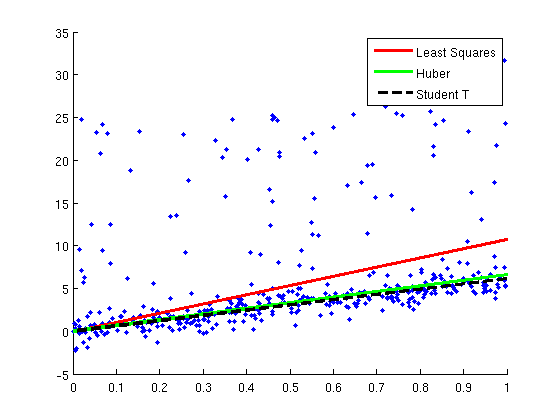
Huber and Student T robust regression

% Generate linear regression data set with outliers
nInstances = 400;
nVars = 1;
[X,y] = makeData('regressionOutliers',nInstances,nVars);

% Least squares solution
wLS = X\y;

% Huber loss
changePoint = .2;
fprintf('Training Huber robust regression model...\n');
wHuber = minFunc(@HuberLoss,wLS,options,X,y,changePoint);

% Student T loss
lambda = 1;
dof = 2;
funObj = @(params)studentLoss(X,y,params(1:nVars),params(nVars+1),params(end));
fprintf('Training student T robust regression model...\n');
params = minFunc(funObj,[wLS;lambda;dof],options);
wT = params(1:nVars);
lambda = params(nVars+1);
dof = params(end);

% Plot results
figure;hold on
plot(X,y,'.');
xl = xlim;
h1=plot(xl,xl*wLS,'r');
h2=plot(xl,xl*wHuber,'g');
h3=plot(xl,xl*wT,'k--');
set(h1,'LineWidth',3);
set(h2,'LineWidth',3);
set(h3,'LineWidth',3);
legend([h1 h2 h3],{'Least Squares','Huber','Student T'});
pause;

Training Huber robust regression model...
Training student T robust regression model...

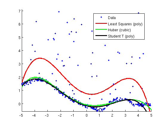
Robust Regression with Basis Expansion

% Generate non-linear regression data set
nInstances = 400;
nVars = 1;
[X,y,ylimits] = makeData('regressionNonlinearOutliers',nInstances,nVars);

% Least squares (cubic polynomial basis)
wLS_poly = [ones(nInstances,1) X X.^2 X.^3 X.^4 X.^5]\y;

% Huber loss (cubic polynomial basis)
fprintf('Training Huber robust polynomial regression model...\n');
wHuber_poly = minFunc(@HuberLoss,[0;0;0;0;0;0],options,[ones(nInstances,1) X X.^2 X.^3 X.^4 X.^5],y,changePoint);

% Student T loss (cubic polynomial basis)
fprintf('Training student T polynomial regression model...\n');
funObj = @(params)studentLoss([ones(nInstances,1) X X.^2 X.^3 X.^4 X.^5],y,params(1:6),params(7),params(end));
wT_poly = minFunc(funObj,[wHuber_poly;lambda;dof],options);
wT_poly = wT_poly(1:6);

% Plot Data
figure;hold on
hD = plot(X,y,'.');

% Plot Regression Functions
Xtest = [-5:.05:5]';
nTest = size(Xtest,1);

hLS_poly = plot(Xtest,[ones(nTest,1) Xtest Xtest.^2 Xtest.^3 Xtest.^4 Xtest.^5]*wLS_poly,'r');
set(hLS_poly,'LineWidth',3);

hHuber_poly = plot(Xtest,[ones(nTest,1) Xtest Xtest.^2 Xtest.^3 Xtest.^4 Xtest.^5]*wHuber_poly,'g');
set(hHuber_poly,'LineWidth',3);

hT_poly = plot(Xtest,[ones(nTest,1) Xtest Xtest.^2 Xtest.^3 Xtest.^4 Xtest.^5]*wT_poly,'k');
set(hT_poly,'LineWidth',3);

legend([hD hLS_poly hHuber_poly, hT_poly],...
    {'Data','Least Squares (poly)',...
	'Huber (cubic)','Student T (poly)'},...
    'Location','Best');
ylim(ylimits);
pause;

Training Huber robust polynomial regression model...
Training student T polynomial regression model...

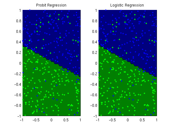
Logistic and Probit regression

% Generate linear classification data set with some variables flipped
nInstances = 400;
nVars = 2;
[X,y] = makeData('classificationFlip',nInstances,nVars);

% Add bias
X = [ones(nInstances,1) X];

fprintf('Training logistic regression model...\n');
wLogistic = minFunc(@LogisticLoss,zeros(nVars+1,1),options,X,y);

trainErr = sum(y ~= sign(X*wLogistic))/length(y)

fprintf('Training probit regression model...\n');
wProbit = minFunc(@ProbitLoss,zeros(nVars+1,1),options,X,y);

trainErr = sum(y ~= sign(X*wProbit))/length(y)

% Plot the result
figure;
subplot(1,2,1);
plotClassifier(X,y,wProbit,'Probit Regression');
subplot(1,2,2);
plotClassifier(X,y,wLogistic,'Logistic Regression');
pause;

Training logistic regression model...

trainErr =

    0.1075

Training probit regression model...

trainErr =

    0.1100

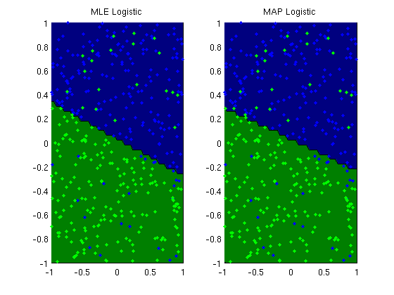
L2-regularized logistic regression

% Find L2-regularized logistic
funObj = @(w)LogisticLoss(w,X,y);
lambda = 10*ones(nVars+1,1);
lambda(1) = 0; % Don't penalize bias
fprintf('Training L2-regularized logistic regression model...\n');
wL2 = minFunc(@penalizedL2,zeros(nVars+1,1),options,funObj,lambda);

trainErr_L2 = sum(y ~= sign(X*wL2))/length(y)

% Plot the result
figure;
subplot(1,2,1);
plotClassifier(X,y,wLogistic,'MLE Logistic');
subplot(1,2,2);
plotClassifier(X,y,wL2,'MAP Logistic');
fprintf('Comparison of norms of parameters for MLE and MAP:\n');
norm_wMLE = norm(wLogistic)
norm_wMAP = norm(wL2)
pause;

Training L2-regularized logistic regression model...

trainErr_L2 =

    0.1175

Comparison of norms of parameters for MLE and MAP:

norm_wMLE =

    3.7901


norm_wMAP =

    1.5583

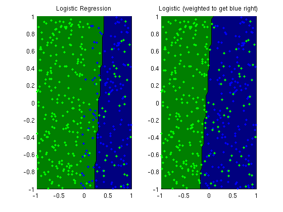
Weighted Logistic regression

% Make a separable data set
nInstances = 400;
nVars = 2;
[X,y] = makeData('classificationFlipOne',nInstances,nVars);

% Add bias
X = [ones(nInstances,1) X];

% Find unweighted maximum likelihood logistic
fprintf('Training unweighted logistic regression model...\n');
wMLE = minFunc(@LogisticLoss,zeros(nVars+1,1),options,X,y);

% Find weighted maximum likelihood logistic
fprintf('Training weighted logistic regression model...\n');
weights = 1+5*(y==-1);
wWeighted = minFunc(@WeightedLogisticLoss,zeros(nVars+1,1),options,X,y,weights);

trainErr_MLE = sum(y ~= sign(X*wMLE))/length(y)
trainErr_weighted = sum(y ~= sign(X*wWeighted))/length(y)

% Plot the result
figure;
subplot(1,2,1);
plotClassifier(X,y,wMLE,'Logistic Regression');
subplot(1,2,2);
plotClassifier(X,y,wWeighted,'Logistic (weighted to get blue right)');
pause;

Training unweighted logistic regression model...
Training weighted logistic regression model...

trainErr_MLE =

    0.1850


trainErr_weighted =

    0.1500

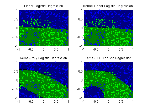
Kernel logistic regression

% Generate non-linear data set
nInstances = 400;
nVars = 2;
[X,y] = makeData('classificationNonlinear',nInstances,nVars);

lambda = 1e-2;

% First fit a regular linear model
funObj = @(w)LogisticLoss(w,X,y);
fprintf('Training linear logistic regression model...\n');
wLinear = minFunc(@penalizedL2,zeros(nVars,1),options,funObj,lambda);

% Now fit the same model with the kernel representation
K = kernelLinear(X,X);
funObj = @(u)LogisticLoss(u,K,y);
fprintf('Training kernel(linear) logistic regression model...\n');
uLinear = minFunc(@penalizedKernelL2,zeros(nInstances,1),options,K,funObj,lambda);

% Now try a degree-2 polynomial kernel expansion
polyOrder = 2;
Kpoly = kernelPoly(X,X,polyOrder);
funObj = @(u)LogisticLoss(u,Kpoly,y);
fprintf('Training kernel(poly) logistic regression model...\n');
uPoly = minFunc(@penalizedKernelL2,zeros(nInstances,1),options,Kpoly,funObj,lambda);

% Squared exponential radial basis function kernel expansion
rbfScale = 1;
Krbf = kernelRBF(X,X,rbfScale);
funObj = @(u)LogisticLoss(u,Krbf,y);
fprintf('Training kernel(rbf) logistic regression model...\n');
uRBF = minFunc(@penalizedKernelL2,zeros(nInstances,1),options,Krbf,funObj,lambda);

% Check that wLinear and uLinear represent the same model:
fprintf('Parameters estimated from linear and kernel(linear) model:\n');
[wLinear X'*uLinear]

trainErr_linear = sum(y ~= sign(X*wLinear))/length(y)
trainErr_poly = sum(y ~= sign(Kpoly*uPoly))/length(y)
trainErr_rbf = sum(y ~= sign(Krbf*uRBF))/length(y)

fprintf('Making plots...\n');
figure;
subplot(2,2,1);
plotClassifier(X,y,wLinear,'Linear Logistic Regression');
subplot(2,2,2);
plotClassifier(X,y,uLinear,'Kernel-Linear Logistic Regression',@kernelLinear,[]);
subplot(2,2,3);
plotClassifier(X,y,uPoly,'Kernel-Poly Logistic Regression',@kernelPoly,polyOrder);
subplot(2,2,4);
plotClassifier(X,y,uRBF,'Kernel-RBF Logistic Regression',@kernelRBF,rbfScale);
pause;

Training linear logistic regression model...
Training kernel(linear) logistic regression model...
Training kernel(poly) logistic regression model...
Training kernel(rbf) logistic regression model...
Parameters estimated from linear and kernel(linear) model:

ans =

   -0.1402   -0.1402
   -1.5940   -1.5940


trainErr_linear =

    0.3025


trainErr_poly =

    0.1400


trainErr_rbf =

    0.0950

Making plots...

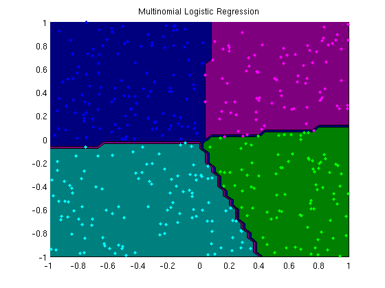
Multinomial logistic regression with L2-regularization

nClasses = 5;
[X,y] = makeData('multinomial',nInstances,nVars,nClasses);

% Add bias
X = [ones(nInstances,1) X];

funObj = @(W)SoftmaxLoss2(W,X,y,nClasses);
lambda = 1e-4*ones(nVars+1,nClasses-1);
lambda(1,:) = 0; % Don't penalize biases
fprintf('Training multinomial logistic regression model...\n');
wSoftmax = minFunc(@penalizedL2,zeros((nVars+1)*(nClasses-1),1),options,funObj,lambda(:));
wSoftmax = reshape(wSoftmax,[nVars+1 nClasses-1]);
wSoftmax = [wSoftmax zeros(nVars+1,1)];

[junk yhat] = max(X*wSoftmax,[],2);
trainErr = sum(yhat~=y)/length(y)

% Plot the result
figure;
plotClassifier(X,y,wSoftmax,'Multinomial Logistic Regression');
pause;

Training multinomial logistic regression model...

trainErr =

    0.0050

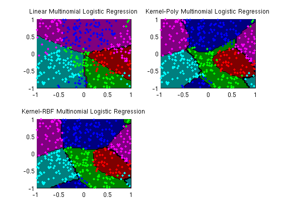
Kernel multinomial logistic regression

% Generate Data
nClasses = 5;
[X,y] = makeData('multinomialNonlinear',nInstances,nVars,nClasses);

lambda = 1e-2;

% Linear
funObj = @(w)SoftmaxLoss2(w,X,y,nClasses);
fprintf('Training linear multinomial logistic regression model...\n');
wLinear = minFunc(@penalizedL2,zeros(nVars*(nClasses-1),1),options,funObj,lambda);
wLinear = reshape(wLinear,[nVars nClasses-1]);
wLinear = [wLinear zeros(nVars,1)];

% Polynomial
polyOrder = 2;
Kpoly = kernelPoly(X,X,polyOrder);
funObj = @(u)SoftmaxLoss2(u,Kpoly,y,nClasses);
fprintf('Training kernel(poly) multinomial logistic regression model...\n');
uPoly = minFunc(@penalizedKernelL2_matrix,randn(nInstances*(nClasses-1),1),options,Kpoly,nClasses-1,funObj,lambda);
uPoly = reshape(uPoly,[nInstances nClasses-1]);
uPoly = [uPoly zeros(nInstances,1)];

% RBF
rbfScale = 1;
Krbf = kernelRBF(X,X,rbfScale);
funObj = @(u)SoftmaxLoss2(u,Krbf,y,nClasses);
fprintf('Training kernel(rbf) multinomial logistic regression model...\n');
uRBF = minFunc(@penalizedKernelL2_matrix,randn(nInstances*(nClasses-1),1),options,Krbf,nClasses-1,funObj,lambda);
uRBF = reshape(uRBF,[nInstances nClasses-1]);
uRBF = [uRBF zeros(nInstances,1)];

% Compute training errors
[junk yhat] = max(X*wLinear,[],2);
trainErr_linear = sum(y~=yhat)/length(y)
[junk yhat] = max(Kpoly*uPoly,[],2);
trainErr_poly = sum(y~=yhat)/length(y)
[junk yhat] = max(Krbf*uRBF,[],2);
trainErr_rbf = sum(y~=yhat)/length(y)

fprintf('Making plots...\n');
figure;
subplot(2,2,1);
plotClassifier(X,y,wLinear,'Linear Multinomial Logistic Regression');
subplot(2,2,2);
plotClassifier(X,y,uPoly,'Kernel-Poly Multinomial Logistic Regression',@kernelPoly,polyOrder);
subplot(2,2,3);
plotClassifier(X,y,uRBF,'Kernel-RBF Multinomial Logistic Regression',@kernelRBF,rbfScale);
pause;

Training linear multinomial logistic regression model...
Training kernel(poly) multinomial logistic regression model...
Training kernel(rbf) multinomial logistic regression model...

trainErr_linear =

    0.3850


trainErr_poly =

    0.1250


trainErr_rbf =

    0.0825

Making plots...

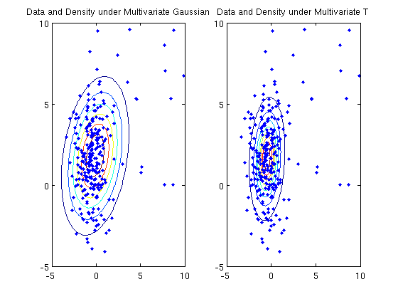
Density estimation with multivariate student T

% Generate data from a Gaussian with outliers
nInstances = 250;
nVars = 2;
nOutliers = 25;
mu = randn(nVars,1);
sigma = randn(nVars);
sigma = sigma+sigma'; % Make symmetric
sigma = sigma + (1-min(eig(sigma)))*eye(nVars);
X = mvnrnd(mu,sigma,nInstances);
X(ceil(rand(nOutliers,1)*nInstances),:) = abs(10*rand(nOutliers,nVars));

% Fit a Gaussian
mu_Gauss = mean(X,1);
sigma_Gauss = cov(X) + 1e-8*eye(nVars);
lik_Gauss = mvnpdf(X,mu_Gauss,sigma_Gauss);

% Fit a multivariate student T
mu_old = ones(nVars,1);
mu = zeros(nVars,1);
%sigma = eye(nVars);
dof = 3;
fprintf('Fitting multivariate student T density model...\n');
while norm(mu-mu_old,'inf') > 1e-4
	mu_old = mu;

	% Update mean
	funObj_mu = @(mu)multivariateT(X,mu,sigma,dof,1);
	mu = minFunc(funObj_mu,mu,options);

	% Update covariance
	funObj_sigma = @(sigma)multivariateT(X,mu,sigma,dof,2);
	sigma(:) = minFunc(funObj_sigma,sigma(:),options);

	% Update dof
	funObj_dof = @(dof)multivariateT(X,mu,sigma,dof,3);
	dof = minFunc(funObj_dof,dof,options);
end
lik_T = multivariateTpdf(X,mu,sigma,dof);
fprintf('log-likelihood under multivariate Gaussian: %f\n',sum(log(lik_Gauss)));
fprintf('log-likelihood under multivariate T: %f\n',sum(log(lik_T)));

% Plot data and densities
figure;
subplot(1,2,1);
plot(X(:,1),X(:,2),'.');
increment = 100;
domain1 = xlim;
domain1 = domain1(1):(domain1(2)-domain1(1))/increment:domain1(2);
domain2 = ylim;
domain2 = domain2(1):(domain2(2)-domain2(1))/increment:domain2(2);
d1 = repmat(domain1',[1 length(domain1)]);
d2 = repmat(domain2,[length(domain2) 1]);
lik_Gauss = mvnpdf([d1(:) d2(:)],mu_Gauss,sigma_Gauss);
contour(d1,d2,reshape(lik_Gauss,size(d1)));hold on;
plot(X(:,1),X(:,2),'.');
title('Data and Density under Multivariate Gaussian');
subplot(1,2,2);
lik_T = multivariateTpdf([d1(:) d2(:)],mu,sigma,dof);
contour(d1,d2,reshape(lik_T,size(d1)));hold on;
plot(X(:,1),X(:,2),'.');
title('Data and Density under Multivariate T');
pause

Fitting multivariate student T density model...
log-likelihood under multivariate Gaussian: -1092.464005
log-likelihood under multivariate T: -1023.382586

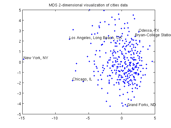
Data Visualization with Multi-Dimensional Scaling

load cities.mat
X = standardizeCols(ratings);
[n,p] = size(X);

% Compute all pairwise distances
X2 = X.^2;
D = sqrt(X2*ones(p,n) + ones(n,p)*X2' - 2*X*X');

% Choose number of components and (random) initialization
nComponents = 2;
z = 1e-16*randn(n,nComponents);

% Turn on visualization
visualize = 1;
fprintf('Running MDS to make 2-dimensional visualization of cities data...\n');
figure;
z(:) = minFunc(@MDSstress,z(:),options,D,visualize);

% Visualize results
title('MDS 2-dimensional visualization of cities data');
fprintf('Click plot to name cities, press any key to continue\n');
gname(names);

Running MDS to make 2-dimensional visualization of cities data...
Click plot to name cities, press any key to continue

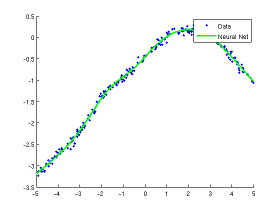
Regression with neural networks

% Generate non-linear regression data set
nVars = 1;
[X,y] = makeData('regressionNonlinear',nInstances,nVars);

X = [ones(nInstances,1) X];
nVars = nVars+1;

% Train neural network
nHidden = [10];
nParams = nVars*nHidden(1);
for h = 2:length(nHidden);
    nParams = nParams+nHidden(h-1)*nHidden(h);
end
nParams = nParams+nHidden(end);

funObj = @(weights)MLPregressionLoss(weights,X,y,nHidden);
lambda = 1e-2;
fprintf('Training neural network for regression...\n');
wMLP = minFunc(@penalizedL2,randn(nParams,1),options,funObj,lambda);

% Plot results
figure;hold on
Xtest = [-5:.05:5]';
Xtest = [ones(size(Xtest,1),1) Xtest];
yhat = MLPregressionPredict(wMLP,Xtest,nHidden);
plot(X(:,2),y,'.');
h=plot(Xtest(:,2),yhat,'g-');
set(h,'LineWidth',3);
legend({'Data','Neural Net'});
pause;

Training neural network for regression...

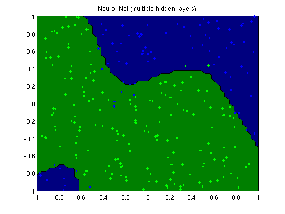
Classification with Neural Network with multiple hidden layers

nVars = 2;
[X,y] = makeData('classificationNonlinear',nInstances,nVars);

X = [ones(nInstances,1) X];
nVars = nVars+1;

% Train neural network w/ multiple hiden layers
nHidden = [10 10];
nParams = nVars*nHidden(1);
for h = 2:length(nHidden);
    nParams = nParams+nHidden(h-1)*nHidden(h);
end
nParams = nParams+nHidden(end);

funObj = @(weights)MLPbinaryLoss(weights,X,y,nHidden);
lambda = 1;
fprintf('Training neural network with multiple hidden layers for classification\n');
wMLP = minFunc(@penalizedL2,randn(nParams,1),options,funObj,lambda);

yhat = MLPregressionPredict(wMLP,X,nHidden);
trainErr = sum(sign(yhat(:)) ~= y)/length(y)

fprintf('Making plot...\n');
figure;
plotClassifier(X,y,wMLP,'Neural Net (multiple hidden layers)',nHidden);
pause;

Training neural network with multiple hidden layers for classification

trainErr =

    0.0560

Making plot...

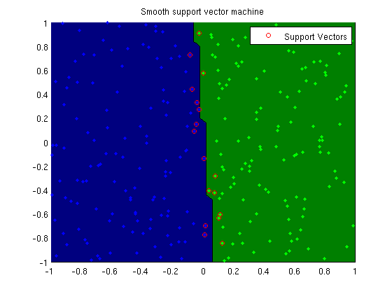
Smooth support vector machine

nVars = 2;
[X,y] = makeData('classification',nInstances,nVars);

% Add bias
X = [ones(nInstances,1) X];

fprintf('Training smooth vector machine model...\n');
funObj = @(w)SSVMLoss(w,X,y);
lambda = 1e-2*ones(nVars+1,1);
lambda(1) = 0;
wSSVM = minFunc(@penalizedL2,zeros(nVars+1,1),options,funObj,lambda);

trainErr = sum(y ~= sign(X*wSSVM))/length(y)

% Plot the result
figure;
plotClassifier(X,y,wSSVM,'Smooth support vector machine');
SV = 1-y.*(X*wSSVM) >= 0;
h=plot(X(SV,2),X(SV,3),'o','color','r');
legend(h,'Support Vectors');
pause;

Training smooth vector machine model...

trainErr =

    0.0040

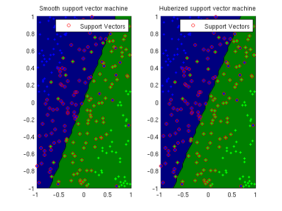
Huberized support vector machine

nVars = 2;
[X,y] = makeData('classificationFlip',nInstances,nVars);

% Add bias
X = [ones(nInstances,1) X];

fprintf('Training smooth support vector machine model...\n');
funObj = @(w)SSVMLoss(w,X,y);
lambda = 1e-2*ones(nVars+1,1);
lambda(1) = 0;
wSSVM = minFunc(@penalizedL2,zeros(nVars+1,1),options,funObj,lambda);

fprintf('Training huberized support vector machine model...\n');
t = .5;
funObj = @(w)HuberSVMLoss(w,X,y,t);
lambda = 1e-2*ones(nVars+1,1);
lambda(1) = 0;
wHSVM = minFunc(@penalizedL2,zeros(nVars+1,1),options,funObj,lambda);

trainErr = sum(y ~= sign(X*wSSVM))/length(y)
trainErr = sum(y ~= sign(X*wHSVM))/length(y)

% Plot the result
figure;
subplot(1,2,1);
plotClassifier(X,y,wSSVM,'Smooth support vector machine');
SV = 1-y.*(X*wSSVM) >= 0;
h=plot(X(SV,2),X(SV,3),'o','color','r');
legend(h,'Support Vectors');
subplot(1,2,2);
plotClassifier(X,y,wHSVM,'Huberized support vector machine');
SV = 1-y.*(X*wSSVM) >= 0;
h=plot(X(SV,2),X(SV,3),'o','color','r');
legend(h,'Support Vectors');
pause;

Training smooth support vector machine model...
Training huberized support vector machine model...

trainErr =

    0.1040


trainErr =

    0.1040

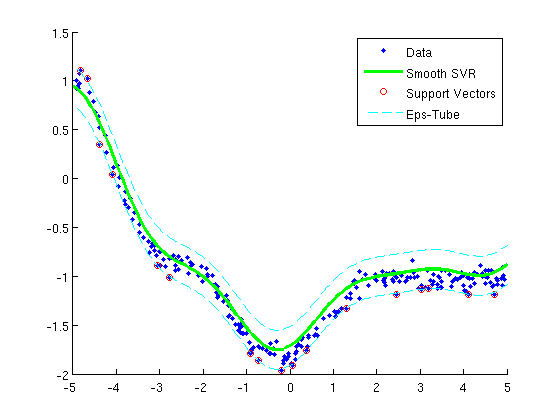
Smooth support vector regression

nVars = 1;
[X,y] = makeData('regressionNonlinear',nInstances,nVars);

X = [ones(nInstances,1) X];
nVars = nVars+1;

lambda = 1e-2;

% Train smooth support vector regression machine
changePoint = .2;
rbfScale = 1;
Krbf = kernelRBF(X,X,rbfScale);
funObj = @(u)SSVRLoss(u,Krbf,y,changePoint);
fprintf('Training kernel(rbf) support vector regression machine...\n');
uRBF = minFunc(@penalizedKernelL2,zeros(nInstances,1),options,Krbf,funObj,lambda);

% Plot results
figure;hold on
plot(X(:,2),y,'.');
Xtest = [-5:.05:5]';
Xtest = [ones(size(Xtest,1),1) Xtest];
yhat = kernelRBF(Xtest,X,rbfScale)*uRBF;
h=plot(Xtest(:,2),yhat,'g-');
set(h,'LineWidth',3);
SV = abs(Krbf*uRBF - y) >= changePoint;
plot(X(SV,2),y(SV),'o','color','r');
plot(Xtest(:,2),yhat+changePoint,'c--');
plot(Xtest(:,2),yhat-changePoint,'c--');
legend({'Data','Smooth SVR','Support Vectors','Eps-Tube'});
pause;

Training kernel(rbf) support vector regression machine...

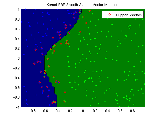
Kernel smooth support vector machine

% Generate non-linear data set
nVars = 2;
[X,y] = makeData('classificationNonlinear',nInstances,nVars);

lambda = 1e-2;

% Squared exponential radial basis function kernel expansion
rbfScale = 1;
Krbf = kernelRBF(X,X,rbfScale);
funObj = @(u)SSVMLoss(u,Krbf,y);
fprintf('Training kernel(rbf) support vector machine...\n');
uRBF = minFunc(@penalizedKernelL2,zeros(nInstances,1),options,Krbf,funObj,lambda);

trainErr = sum(y ~= sign(Krbf*uRBF))/length(y)

fprintf('Making plot...\n');
figure;
plotClassifier(X,y,uRBF,'Kernel-RBF Smooth Support Vector Machine',@kernelRBF,rbfScale);
SV = 1-y.*(Krbf*uRBF) >= 0;
h=plot(X(SV,1),X(SV,2),'o','color','r');
legend(h,'Support Vectors');
pause;

Training kernel(rbf) support vector machine...

trainErr =

    0.0480

Making plot...

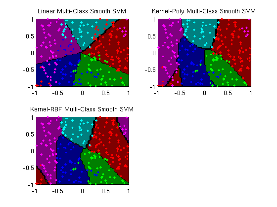
Multi-class smooth support vector machine

% Generate Data
nVars = 2;
nClasses = 5;
[X,y] = makeData('multinomialNonlinear',nInstances,nVars,nClasses);

lambda = 1e-2;

% Linear
funObj = @(w)SSVMMultiLoss(w,X,y,nClasses);
fprintf('Training linear multi-class SVM...\n');
wLinear = minFunc(@penalizedL2,zeros(nVars*nClasses,1),options,funObj,lambda);
wLinear = reshape(wLinear,[nVars nClasses]);

% Polynomial
polyOrder = 2;
Kpoly = kernelPoly(X,X,polyOrder);
funObj = @(u)SSVMMultiLoss(u,Kpoly,y,nClasses);
fprintf('Training kernel(poly) multi-class SVM...\n');
uPoly = minFunc(@penalizedKernelL2_matrix,randn(nInstances*nClasses,1),options,Kpoly,nClasses,funObj,lambda);
uPoly = reshape(uPoly,[nInstances nClasses]);

% RBF
rbfScale = 1;
Krbf = kernelRBF(X,X,rbfScale);
funObj = @(u)SSVMMultiLoss(u,Krbf,y,nClasses);
fprintf('Training kernel(rbf) multi-class SVM...\n');
uRBF = minFunc(@penalizedKernelL2_matrix,randn(nInstances*nClasses,1),options,Krbf,nClasses,funObj,lambda);
uRBF = reshape(uRBF,[nInstances nClasses]);

% Compute training errors
[junk yhat] = max(X*wLinear,[],2);
trainErr_linear = sum(y~=yhat)/length(y)
[junk yhat] = max(Kpoly*uPoly,[],2);
trainErr_poly = sum(y~=yhat)/length(y)
[junk yhat] = max(Krbf*uRBF,[],2);
trainErr_rbf = sum(y~=yhat)/length(y)

fprintf('Making plots...\n');
figure;
subplot(2,2,1);
plotClassifier(X,y,wLinear,'Linear Multi-Class Smooth SVM');
subplot(2,2,2);
plotClassifier(X,y,uPoly,'Kernel-Poly Multi-Class Smooth SVM',@kernelPoly,polyOrder);
subplot(2,2,3);
plotClassifier(X,y,uRBF,'Kernel-RBF Multi-Class Smooth SVM',@kernelRBF,rbfScale);
pause;

Training linear multi-class SVM...
Training kernel(poly) multi-class SVM...
Training kernel(rbf) multi-class SVM...

trainErr_linear =

    0.3560


trainErr_poly =

    0.1400


trainErr_rbf =

    0.0800

Making plots...

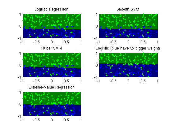
Extreme-value regression

% Make a separable data set
nInstances = 200;
nVars = 2;
[X,y] = makeData('classificationFlipOne',nInstances,nVars);

% Add bias
X = [ones(nInstances,1) X];

% Fit unweighted maximum likelihood logistic
fprintf('Training unweighted logistic regression model...\n');
wlogistic = minFunc(@LogisticLoss,zeros(nVars+1,1),options,X,y);

% Fit smooth SVM
fprintf('Training smooth SVM...\n');
wSSVM = minFunc(@SSVMLoss,zeros(nVars+1,1),options,X,y);

% Fit huberized SVM (almost the same as regular non-smooth SVM)
fprintf('Training huberized SVM...\n');
wHSVM = minFunc(@HuberSVMLoss,randn(nVars+1,1),options,X,y,.5);

% Fit weighted maximum likelihood logistic
fprintf('Training weighted logistic regression model...\n');
weights = 1+5*(y==-1);
wWeighted = minFunc(@WeightedLogisticLoss,zeros(nVars+1,1),options,X,y,weights);

% Fit extreme-value regression
fprintf('Training extreme-value regression model...\n');
wExtreme = minFunc(@ExtremeLoss,zeros(nVars+1,1),options,X,y);

trainErr_logistic = sum(y ~= sign(X*wlogistic))/length(y)
trainErr_ssvm = sum(y ~= sign(X*wSSVM))/length(y)
trainErr_hsvm = sum(y ~= sign(X*wHSVM))/length(y)
trainErr_weighted = sum(y ~= sign(X*wWeighted))/length(y)
trainErr_extreme = sum(y ~= sign(X*wExtreme))/length(y)

% Plot the result
figure;
subplot(3,2,1);
plotClassifier(X,y,wlogistic,'Logistic Regression');
subplot(3,2,2);
plotClassifier(X,y,wSSVM,'Smooth SVM');
subplot(3,2,3);
plotClassifier(X,y,wHSVM,'Huber SVM');
subplot(3,2,4);
plotClassifier(X,y,wWeighted,'Logistic (blue have 5x bigger weight)');
subplot(3,2,5);
plotClassifier(X,y,wExtreme,'Extreme-Value Regression');
pause;

Training unweighted logistic regression model...
Training smooth SVM...
Training huberized SVM...
Training weighted logistic regression model...
Training extreme-value regression model...

trainErr_logistic =

    0.2000


trainErr_ssvm =

    0.1900


trainErr_hsvm =

    0.1700


trainErr_weighted =

    0.2000


trainErr_extreme =

    0.1500

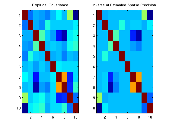
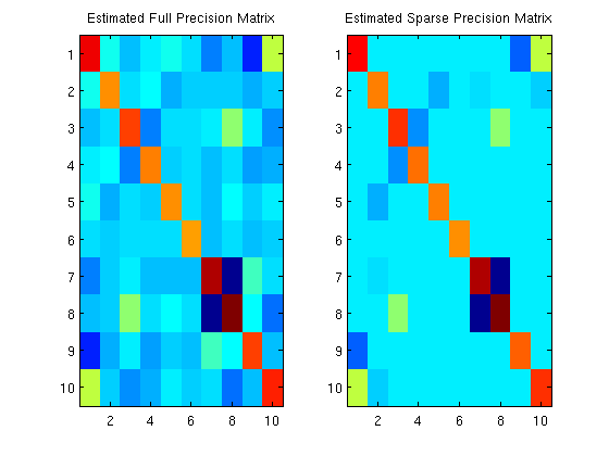
Sparse Gaussian graphical model precision matrix estimation

% Generate a sparse positive-definite precision matrix
nNodes = 10;
adj = triu(rand(nNodes) > .75,1);
adj = setdiag(adj+adj',1);
P = randn(nNodes).*adj;
P = (P+P')/2;
tau = 1;
X = P + tau*eye(nNodes);
while ~ispd(X)
    tau = tau*2;
    X = P + tau*eye(nNodes);
end
mu = randn(nNodes,1);

% Sample from the GGM
C = inv(X);
R = chol(C)';
X = zeros(nInstances,nNodes);
for i = 1:nInstances
    X(i,:) = (mu + R*randn(nNodes,1))';
end

% Center and Standardize
X = standardizeCols(X);

% Train Full GGM
sigma_emp = cov(X);
nonZero = find(ones(nNodes));
funObj = @(x)sparsePrecisionObj(x,nNodes,nonZero,sigma_emp);
Kfull = eye(nNodes);
fprintf('Fitting full Gaussian graphical model\n');
Kfull(nonZero) = minFunc(funObj,Kfull(nonZero),options);

% Train GGM with sparsity pattern given by 'adj'
nonZero = find(adj);
funObj = @(x)sparsePrecisionObj(x,nNodes,nonZero,sigma_emp);
Ksparse = eye(nNodes);
fprintf('Fitting sparse Gaussian graphical model\n');
Ksparse(nonZero) = minFunc(funObj,Ksparse(nonZero),options);

% Covariance matrix corresponding to sparse precision should agree with
% empirical covariance at all non-zero values
fprintf('Norm of difference between empirical and estimated covariance\nmatrix at values where the precision matrix was not set to 0:\n');
Csparse = inv(Ksparse);
norm(sigma_emp(nonZero)-Csparse(nonZero))

figure;
subplot(1,2,1);
imagesc(sigma_emp);
title('Empirical Covariance');
subplot(1,2,2);
imagesc(Csparse);
title('Inverse of Estimated Sparse Precision');
figure;
subplot(1,2,1);
imagesc(Kfull);
title('Estimated Full Precision Matrix');
subplot(1,2,2);
imagesc(Ksparse);
title('Estimated Sparse Precision Matrix');
pause;

Fitting full Gaussian graphical model
Fitting sparse Gaussian graphical model
Norm of difference between empirical and estimated covariance
matrix at values where the precision matrix was not set to 0:

ans =

   7.8088e-06

Chain-structured conditional random field

% Generate Data
nWords = 1000;
nStates = 4;
nFeatures = [2 3 4 5]; % When inputting a data set, this can be set to maximum values in columns of X

% Generate Features (0 means no feature)
clear X
for feat = 1:length(nFeatures)
    X(:,feat) = floor(rand(nWords,1)*(nFeatures(feat)+1));
end

% Generate Labels (0 means position between sentences)
y = floor(rand*(nStates+1));
for w = 2:nWords
    pot = zeros(5,1);

    % Features increase the probability of transitioning to their state
    pot(2) = sum(X(w,:)==1);
    pot(3) = 10*sum(X(w,:)==2);
    pot(4) = 100*sum(X(w,:)==3);
    pot(5) = 1000*sum(X(w,:)==4);

    % We have at least a 10% chance of staying in the same state
    pot(y(w-1,1)+1) = max(pot(y(w-1,1)+1),max(pot)/10);

    % We have a 10% chance of ending the sentence if last state was 1-3, 50% if
    % last state was 4
    if y(w-1) == 0
        pot(1) = 0;
    elseif y(w-1) == 4
        pot(1) = max(pot)/2;
    else
        pot(1) = max(pot)/10;
    end

    pot = pot/sum(pot);
    y(w,1) = sampleDiscrete(pot)-1;
end

% Initialize
[w,v_start,v_end,v] = crfChain_initWeights(nFeatures,nStates,'zeros');
featureStart = cumsum([1 nFeatures(1:end)]); % data structure which relates high-level 'features' to elements of w
sentences = crfChain_initSentences(y);
nSentences = size(sentences,1);
maxSentenceLength = 1+max(sentences(:,2)-sentences(:,1));

fprintf('Training chain-structured CRF\n');
[wv] = minFunc(@crfChain_loss,[w(:);v_start;v_end;v(:)],options,X,y,nStates,nFeatures,featureStart,sentences);

% Split up weights
[w,v_start,v_end,v] = crfChain_splitWeights(wv,featureStart,nStates);

% Measure error
trainErr = 0;
trainZ = 0;
yhat = zeros(size(y));
for s = 1:nSentences
    y_s = y(sentences(s,1):sentences(s,2));
    [nodePot,edgePot]=crfChain_makePotentials(X,w,v_start,v_end,v,nFeatures,featureStart,sentences,s);
    [nodeBel,edgeBel,logZ] = crfChain_infer(nodePot,edgePot);
    [junk yhat(sentences(s,1):sentences(s,2))] = max(nodeBel,[],2);
end
trainErrRate = sum(y~=yhat)/length(y)

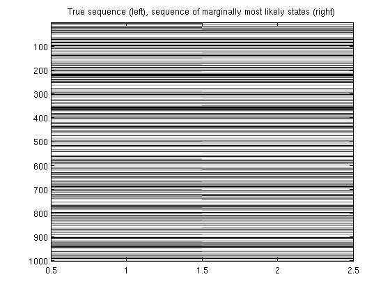
figure;
imagesc([y yhat]);
colormap gray
title('True sequence (left), sequence of marginally most likely states (right)');
pause;

Training chain-structured CRF

trainErrRate =

    0.0920

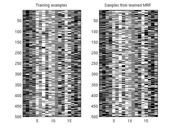
Tree-structured Markov random field with exp(linear) potentials

nInstances = 500;
nNodes = 18;
nStates = 3;

% Make tree-structured adjacency matrix
adj = zeros(nNodes);
adj(1,2) = 1;
adj(1,3) = 1;
adj(1,4) = 1;
adj(2,5) = 1;
adj(2,6) = 1;
adj(2,7) = 1;
adj(3,8) = 1;
adj(7,9) = 1;
adj(7,10) = 1;
adj(8,11) = 1;
adj(8,12) = 1;
adj(8,13) = 1;
adj(8,14) = 1;
adj(9,15) = 1;
adj(9,16) = 1;
adj(9,17) = 1;
adj(13,18) = 1;
adj = adj+adj';

% Make edgeStruct
useMex = 1;
edgeStruct = UGM_makeEdgeStruct(adj,nStates,useMex,nInstances);
nEdges = edgeStruct.nEdges;

% Make potentials and sample from MRF
nodePot = rand(nNodes,nStates);
edgePot = rand(nStates,nStates,nEdges);
y = UGM_Sample_Tree(nodePot,edgePot,edgeStruct)';
y = int32(y);

% Now fit untied MRF with exp(linear) parameters to data
nodeMap = zeros(nNodes,nStates,'int32');
nodeMap(:) = 1:numel(nodeMap);
edgeMap = zeros(nStates,nStates,nEdges,'int32');
edgeMap(:) = numel(nodeMap)+1:numel(nodeMap)+numel(edgeMap);
nParams = max([nodeMap(:);edgeMap(:)]);
w = zeros(nParams,1);
suffStat = UGM_MRF_computeSuffStat(y,nodeMap,edgeMap,edgeStruct);
fprintf('Training tree-structured Markov random field\n');
funObj = @(w)UGM_MRF_NLL(w,nInstances,suffStat,nodeMap,edgeMap,edgeStruct,@UGM_Infer_Tree);
w = minFunc(funObj,w,options);

% Generate Samples from model
[nodePot,edgePot] = UGM_MRF_makePotentials(w,nodeMap,edgeMap,edgeStruct);
ySimulated = UGM_Sample_Tree(nodePot,edgePot,edgeStruct)';

% Plot real vs. simulated data
figure;
subplot(1,2,1);
imagesc(y);
title('Training examples');
colormap gray
subplot(1,2,2);
imagesc(ySimulated);
colormap gray
title('Samples from learned MRF');
pause;

Training tree-structured Markov random field

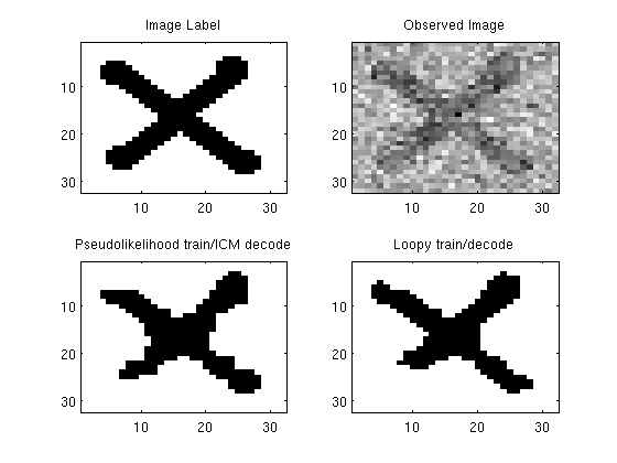
Lattice-structured conditional random field

nInstances = 1;

% Load image/label data
label = sign(double(imread('misc/X.PNG'))-1);
label  = label(:,:,1);
[nRows nCols] = size(label);
noisy = label+randn(nRows,nCols);

% Convert to UGM feature/label format
nNodes = nRows*nCols;
X = reshape(noisy,[nInstances 1 nNodes]);
y = reshape(label,[nInstances nNodes]);

% Standardize Features
tied = 1;
X = UGM_standardizeCols(X,tied);

% Convert from {-1,1} to {1,2} label representation
y(y==1) = 2;
y(y==-1) = 1;
y = int32(y);

% Make adjacency matrix
adjMatrix = latticeAdjMatrix(nRows,nCols);

% Make edges from adjacency matrix
useMex = 1;
nStates = 2;
edgeStruct=UGM_makeEdgeStruct(adjMatrix,nStates,useMex);

% Make edge features
Xedge = UGM_makeEdgeFeatures(X,edgeStruct.edgeEnds);
nEdges = edgeStruct.nEdges;

% Add bias to each node and edge
X = [ones(nInstances,1,nNodes) X];
Xedge = [ones(nInstances,1,nEdges) Xedge];
nNodeFeatures = size(X,2);
nEdgeFeatures = size(Xedge,2);

% Make nodeMap and edgeMap
nodeMap = zeros(nNodes, nStates,nNodeFeatures,'int32');
for f = 1:nNodeFeatures
	nodeMap(:,1,f) = f;
end
edgeMap = zeros(nStates,nStates,nEdges,nEdgeFeatures,'int32');
for edgeFeat = 1:nEdgeFeatures
	for s = 1:nStates
		edgeMap(s,s,:,edgeFeat) = f+edgeFeat;
	end
end
nParams = max([nodeMap(:);edgeMap(:)]);

w = zeros(nParams,1);
funObj = @(w)UGM_CRF_PseudoNLL(w,X,Xedge,y,nodeMap,edgeMap,edgeStruct);
w = minFunc(funObj,w);

[nodePot,edgePot] = UGM_CRF_makePotentials(w,X,Xedge,nodeMap,edgeMap,edgeStruct,1);
y_ICM = UGM_Decode_ICM(nodePot,edgePot,edgeStruct);

fprintf('Training with loopy belief propagation\n');
funObj = @(w)UGM_CRF_NLL(w,X,Xedge,y,nodeMap,edgeMap,edgeStruct,@UGM_Infer_LBP);
w2 = minFunc(funObj,zeros(nParams,1),options);
[nodePot,edgePot] = UGM_CRF_makePotentials(w,X,Xedge,nodeMap,edgeMap,edgeStruct,1);
nodeBel = UGM_Infer_LBP(nodePot,edgePot,edgeStruct);
[junk y_LBP] = max(nodeBel,[],2);

figure;
subplot(2,2,1);
imagesc(label);
colormap gray
title('Image Label');
subplot(2,2,2);
imagesc(noisy);
colormap gray
title('Observed Image');
subplot(2,2,3);
imagesc(reshape(y_ICM,[nRows nCols]));
colormap gray
title('Pseudolikelihood train/ICM decode');
subplot(2,2,4);
imagesc(reshape(y_LBP,[nRows nCols]));
colormap gray
title('Loopy train/decode');

 Iteration   FunEvals     Step Length    Function Val        Opt Cond
         1          2     4.07499e-04     1.59736e+02     2.19437e+02
         2          3     1.00000e+00     1.35716e+02     1.45130e+02
         3          4     1.00000e+00     1.05737e+02     6.02542e+01
         4          5     1.00000e+00     8.93290e+01     3.27338e+01
         5          6     1.00000e+00     7.47799e+01     1.86139e+01
         6          7     1.00000e+00     6.62745e+01     8.34472e+00
         7          8     1.00000e+00     6.36760e+01     1.09284e+01
         8          9     1.00000e+00     6.13427e+01     2.38990e+00
         9         10     1.00000e+00     6.09789e+01     1.74014e+00
        10         11     1.00000e+00     6.07894e+01     1.17248e+00
        11         12     1.00000e+00     6.06990e+01     1.76301e+00
        12         13     1.00000e+00     6.06596e+01     5.95270e-01
        13         14     1.00000e+00     6.06508e+01     1.16771e-01
        14         15     1.00000e+00     6.06501e+01     9.61803e-02
        15         16     1.00000e+00     6.06494e+01     5.79077e-02
        16         17     1.00000e+00     6.06491e+01     1.56045e-02
        17         18     1.00000e+00     6.06490e+01     6.62629e-03
        18         19     1.00000e+00     6.06490e+01     9.54795e-04
        19         20     1.00000e+00     6.06490e+01     1.03171e-04
Directional Derivative below progTol
Training with loopy belief propagation

Published with MATLAB® 7.12