Variational UGM Demo
We have now considered simple local methods for approximate decoding and approximate sampling. In this demo we consider methods that use local computation for approximate inference. We first consider the mean field method, a simple method that iteratively improves a set of marginal estimates. We then consider the loopy belief propagation algorithm, the result of iteratively applying the belief propagation algorithm to a graph with loops. While ICM was a simple example of a local search algorithm and Gibbs sampling is a simple example of an MCMC algorithm, these are simple examples of variational inference algorithms. In addition to these simple variational inference methods, this demo also considers the tree-reweighted variational inference algorithm and variational MCMC methods.
Mean Field Variational Inference
Mean field variational inference algorithms were originally explored in statistical physics. In these methods, we build an approximation of the UGM using a simpler UGM where marginals are easy to compute, but we try to optimize the parameters of the simpler UGM to minimize the Kullback-Leibler divergence from the full UGM. The naive choice for the simpler UGM is a UGM with no edges, and in this case the (normalized) node potentials directly correspond to node marginals. Beginning from some initial guess for each of the node's marginals, the algorithm iterates through the nodes and replaces the current marginals with the (normalized) product of the node potentials and a weighted geometric mean of the corresponding edge potentials, where the weights in the geometric mean are given by the estimates of the marginals of the corresponding neighbors.
Since the nodes are independent in the simpler UGM the approximate edge marginals are given by the product of the relevant node marginals, while the Gibbs mean field free energy gives a lower bound on the normalizing constant. To use the naive mena field method for approximate inference with UGM, you can use:
[nodeBelMF,edgeBelMF,logZMF] = UGM_Infer_MeanField(nodePot,edgePot,edgeStruct);
An example of the marginals computed by the mean field method for a sample of the noisy X problem is:

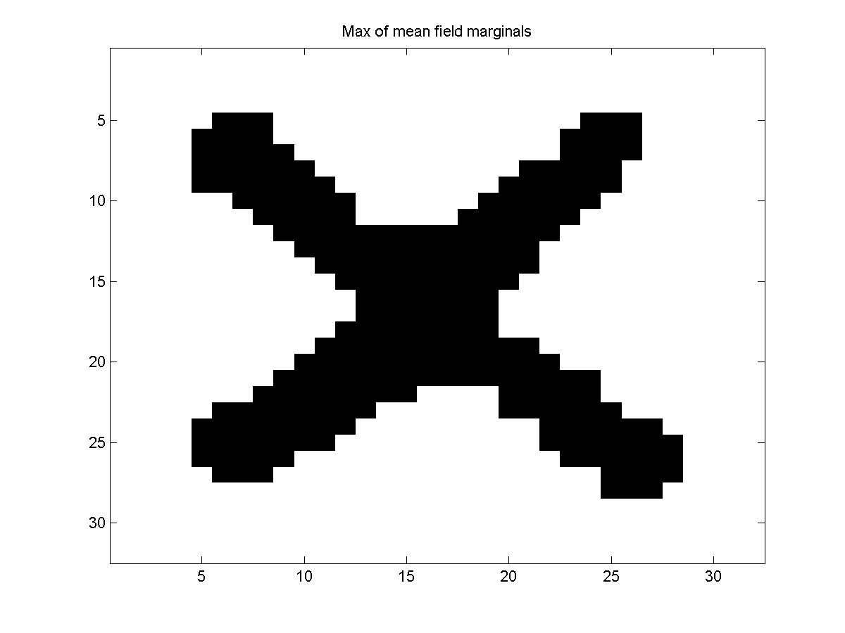
We can also consider taking the maximum of the marginals as an approximate decoding:
maxOfMarginalsMFdecode = UGM_Decode_MaxOfMarginals(nodePot,edgePot,edgeStruct,@UGM_Infer_MeanField);
This yields the following result:
Loopy Belief Propagation
Another widely-used method for approximate inference is the loopy belief propagation algorithm. The idea behind this method is simple; starting from some initial set of belief propagation 'messages', we iterate through our nodes and we repeatedly apply the belief propagation updates to the messages, even though our graph structure is not a tree. This seemingly heuristic method is often surprisingly effective at estimating marginals, and indeed it can be also be viewed as a variational method.
In particular, it can be shown that if these updates converge that they will converge to a fixed point of the Bethe free energy (an approximation of -logZ).
A reference describing the mean field method and loopy belief propagation and their implementations as local message passing algorithms is:
- Y. Weiss. Comparing the mean field method and belief propagation for approximate inference in MRFs. In: Saad and Opper (ed), Advanced Mean Field Methods, 2001.
To use loopy belief propagation for approximate inference, you can use:
[nodeBelLBP,edgeBelLBP,logZLBP] = UGM_Infer_LBP(nodePot,edgePot,edgeStruct);
This gives the following marginals:

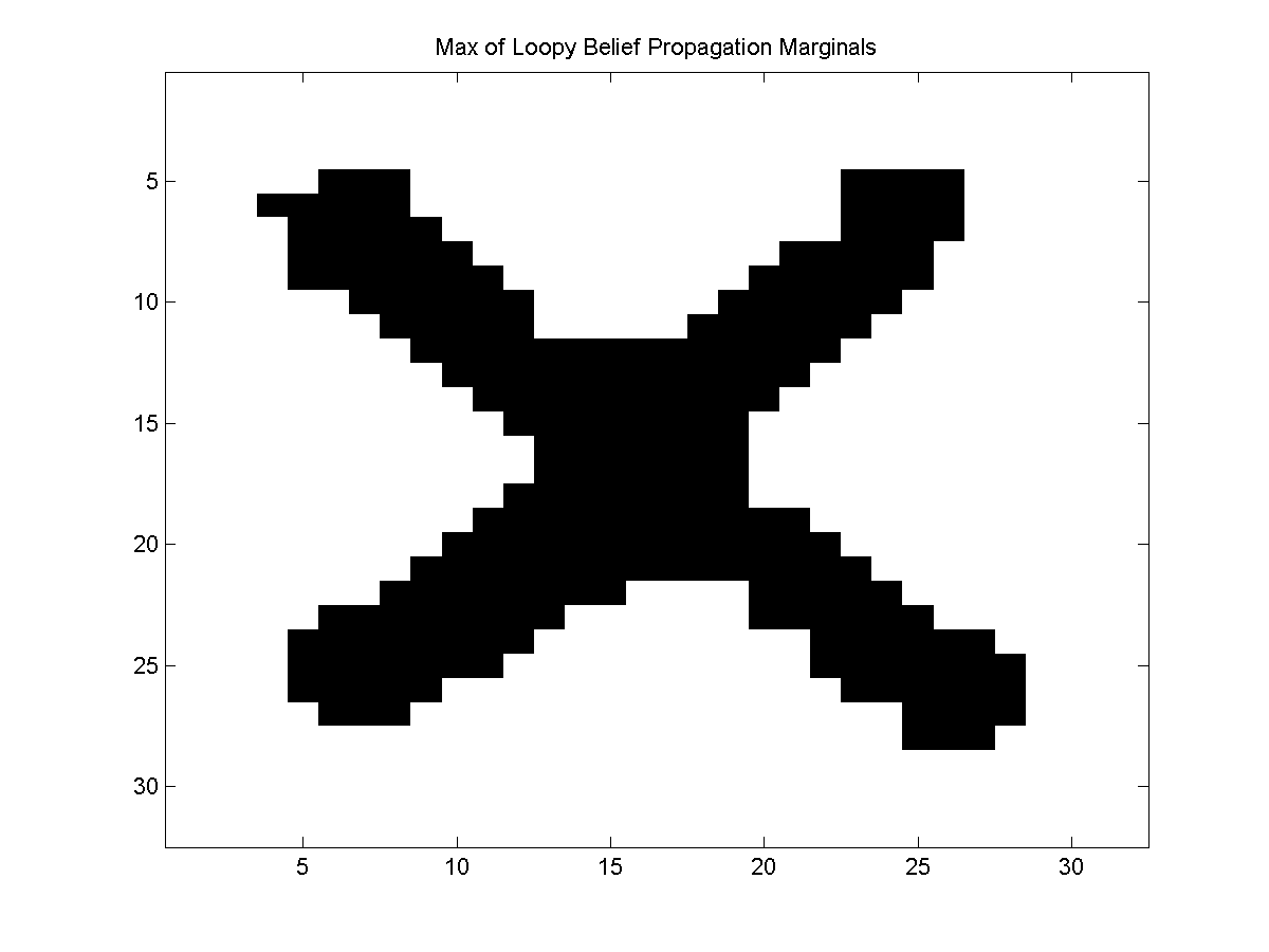
We can obtain the maximum of the marginals using:
maxOfMarginalsLBPdecode = UGM_Decode_MaxOfMarginals(nodePot,edgePot,edgeStruct,@UGM_Infer_LBP);
This yields:
In the case of loopy belief propagation, we can also consider applying the messages used in the decoding version of belief propagation as an approximate decoding method (sometimes called 'max-product' loopy belief propagation, instead of 'sum-product' loopy belief propagation). We can do this with UGM using:
decodeLBP = UGM_Decode_LBP(nodePot,edgePot,edgeStruct);
This yields the result:

Tree-Reweighted Belief Propagation
When using an approximate inference method for parameter estimation, we would like our estimate of -logZ to be an upper bound, and be convex. Unfortunately, neither of the above methods have either of these properties.
However, there has been substantial recent work on variations of the Bethe free energy that have both of these properties. UGM implements one of these variations, tree-reweighted belief propagation.
In the tree-reweighted belief propagation method, the log partition function is upper bounded by a convex combination of tree-structured distributions. Indeed, we might use a very large number of tree-structured distributions in the bound. However, the most interesting part about this method is that we don't need to store the individual distributions. As long as we know the proportion of trees that each edge appears in (and we are careful that each edge appears in at least one tree), we can optimize the bound using an algorithm that is very similar to loopy belief propagation that incorporates these proportions.
The method is described in detail in:
- M.J. Wainwright, T.S. Jakkola, A.S. Willsky. A new class of upper bounds on the log partition function. Uncertainty in Artificial Intelligence, 2002.
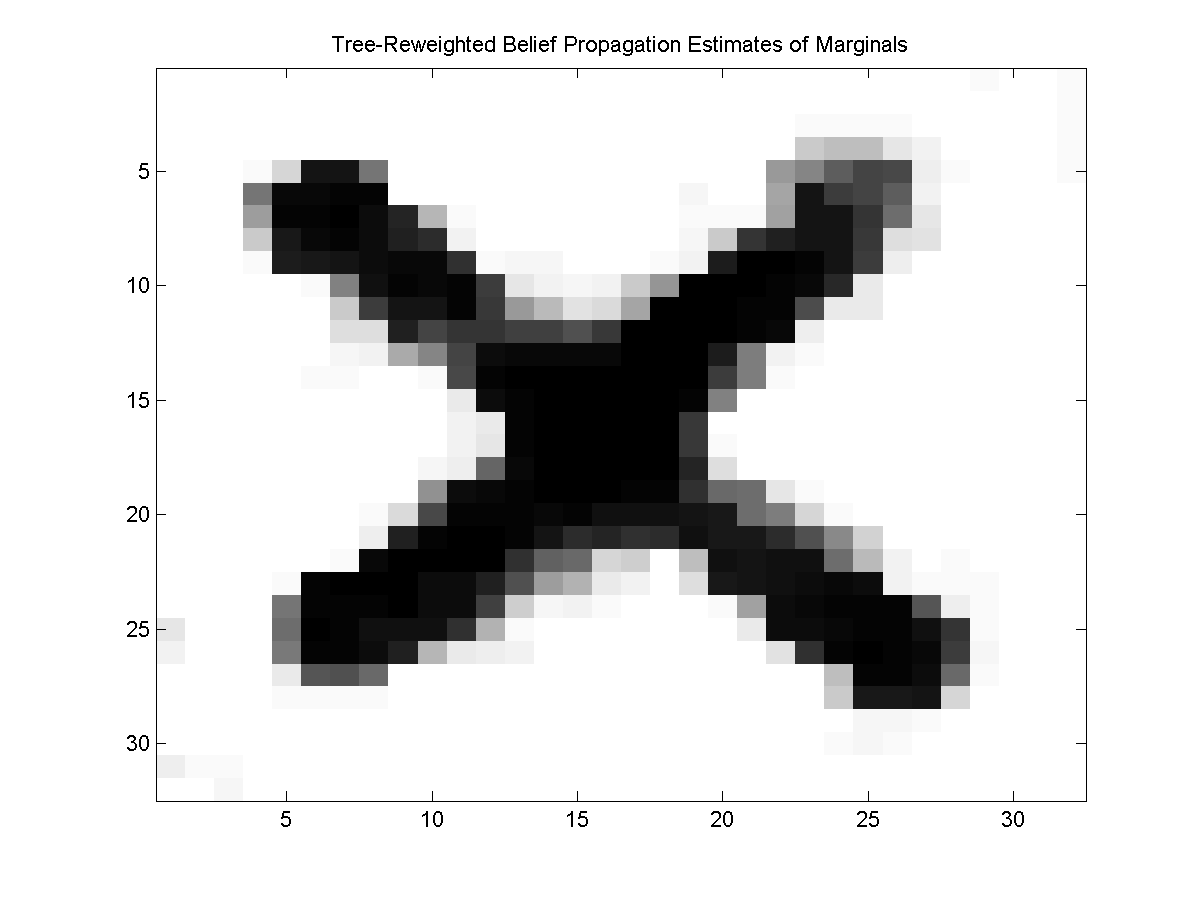
The UGM tree-reweighted belief propagation methods compute the edge proportions by generating random spanning trees until each edge has been included in at least one tree (an alternative set of edge proportions can be specified as an optional fourth argument to UGM_Infer_TRBP). We can call the tree-reweighted belief propagation method for inference in UGM using:
[nodeBelTRBP,edgeBelTRBP,logZTRBP] = UGM_Infer_TRBP(nodePot,edgePot,edgeStruct);
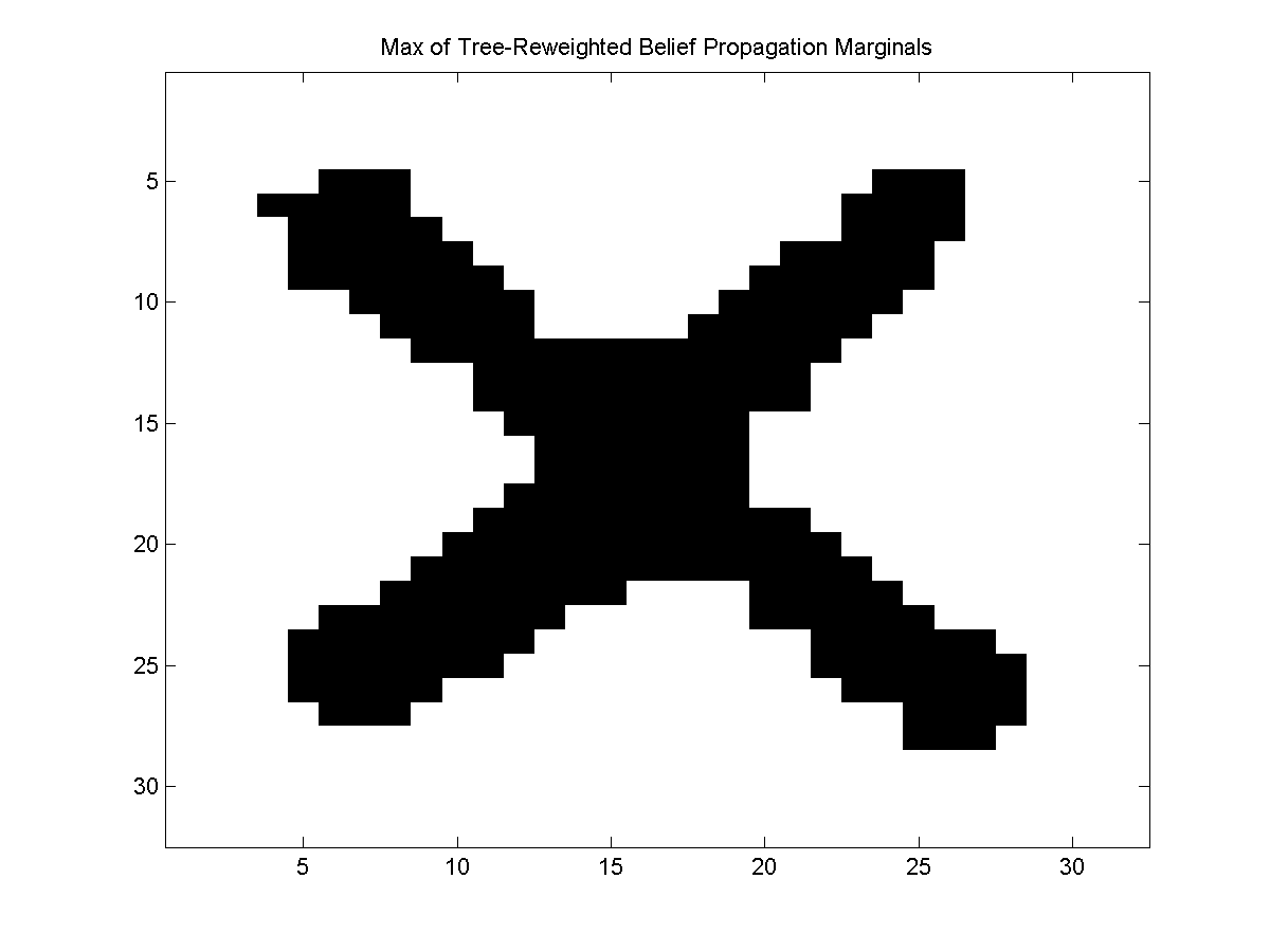
We can similarly call the max of marginals, and decoding version of tree-reweighted belief propagation to yield the following:

Variational MCMC
In the mean field method, we try to optimize the divergence between our UGM and a simple UGM where calculations are easy. Note that it is easy to draw samples from the independent UGM, so if the simple UGM is a good approximation of the full UGM then we might consider using the simple UGM to generate proposals within a Metropolis-Hastings approximate sampling method. This is called variational MCMC and is described in:
- N. de Freitas, P. Hojen-Sorensen, M. Jordan, and S. Russell. Variational MCMC. Uncertainty in Artificial Intelligence, 2001.
As opposed to Gibbs proposals that only change one variable at a time, the variational proposals change all variables at once and may be able to jump between very different parts of the state space. To call a variational MCMC sampler with a burn-in of 100 to generate 100 samples in UGM, you can use:
burnIn = 100;
edgeStruct.maxIter = 100;
variationalProportion = .25;
samplesVarMCMC = UGM_Sample_VarMCMC(nodePot,edgePot,edgeStruct,burnIn,variationalProportion);
The variationalProportion sets the proportion of the iterations where a variational proposal is used (the other iterations use a Gibbs proposal for each variable). Variational MCMC isn't particularly effective for the noisy X problem (the variational proposals are almost always rejected), but its ability to make more global moves might be effective for other problems.
Notes
Variational inference methods remain an active topic of research, and several extensions of the above methods are possible. For example, the above algorithms are not guaranteed to converge to a fixed point and several authors have proposed convergent variational message passing algorithms. It is also possible to use more clever edge proportions in the tree-reweighted methods, or to try and optimize these values.
Notable generalizations of the Bethe approximation to the partition function include methods based on truncated loop series expansions of the partition function, methods based on Kikuchi free energies (this is analogous to the Bethe free energy for a junction tree), and expectation propagation methods. An excellent reference that discusses the world of variational methods is:
- M.J. Wainwright and M. Jordan. Graphical models, exponential families, and variational inference. Foundations and Trends in Machine Learning, 2008.
PREVIOUS DEMO NEXT DEMO
Mark Schmidt > Software > UGM > Variational Demo