Lab 4: PID Control and Virtual Wall
In this lab, we describe how a PID controller is tuned. We describe the effects of each individual terms in the PID controller (i.e. Proportional, Integral and Derivative terms). We describe an implementation of a virtual wall as a one sided spring. We also describe effects of changing sampling rates and introducing delays in the control loop.Proportional Controller
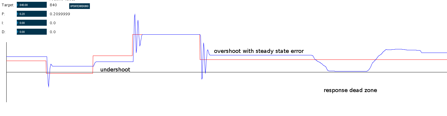 Fig 1. Low Proportional Gain Constant
Figure 1 shows a proportional controller with low proportional gain. Since the gain is only Kp = 0.2, the gain is not enough to compensate for low errors. For example, when the set point was changed to a slightly different value than before, the system reacted like underdamped and did not reach the set point. We call this an undershoot. But for a relatively larger error between current position and target position, the controller would respond with an overshoot, followed by steady state error. The overshoot reflects the effect of proportional gain while the steady state error shows that the proportional gain is still not high enough to compensate for the low offset between current position and target position. We then introduce perturbance on the Twiddler with our hands and observe that the controller only shows any effect only when we push the Twiddler off from the target point enough that the effect of low P would kick in. We call this the response dead zone.
Fig 1. Low Proportional Gain Constant
Figure 1 shows a proportional controller with low proportional gain. Since the gain is only Kp = 0.2, the gain is not enough to compensate for low errors. For example, when the set point was changed to a slightly different value than before, the system reacted like underdamped and did not reach the set point. We call this an undershoot. But for a relatively larger error between current position and target position, the controller would respond with an overshoot, followed by steady state error. The overshoot reflects the effect of proportional gain while the steady state error shows that the proportional gain is still not high enough to compensate for the low offset between current position and target position. We then introduce perturbance on the Twiddler with our hands and observe that the controller only shows any effect only when we push the Twiddler off from the target point enough that the effect of low P would kick in. We call this the response dead zone.
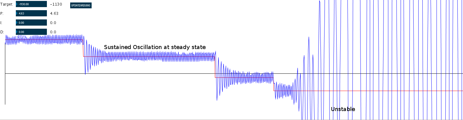 Fig 2. High Proportional Gain Constant
Now, to improve the response of the system at dead zones, we can increase the proportional gain. In figure 2, we show an example with Kp = 4.63. Now, we observe that the system has oscillatory transient response. When the system comes close to the target position, the Kp term is high such that the system starts to oscillate. Watch out, if things go bad, the system could easily go unstable as shown in the figure.
See video here: http://www.youtube.com/watch?v=2-08aaWPc2M&feature=youtu.be
Fig 2. High Proportional Gain Constant
Now, to improve the response of the system at dead zones, we can increase the proportional gain. In figure 2, we show an example with Kp = 4.63. Now, we observe that the system has oscillatory transient response. When the system comes close to the target position, the Kp term is high such that the system starts to oscillate. Watch out, if things go bad, the system could easily go unstable as shown in the figure.
See video here: http://www.youtube.com/watch?v=2-08aaWPc2M&feature=youtu.bePD Controller
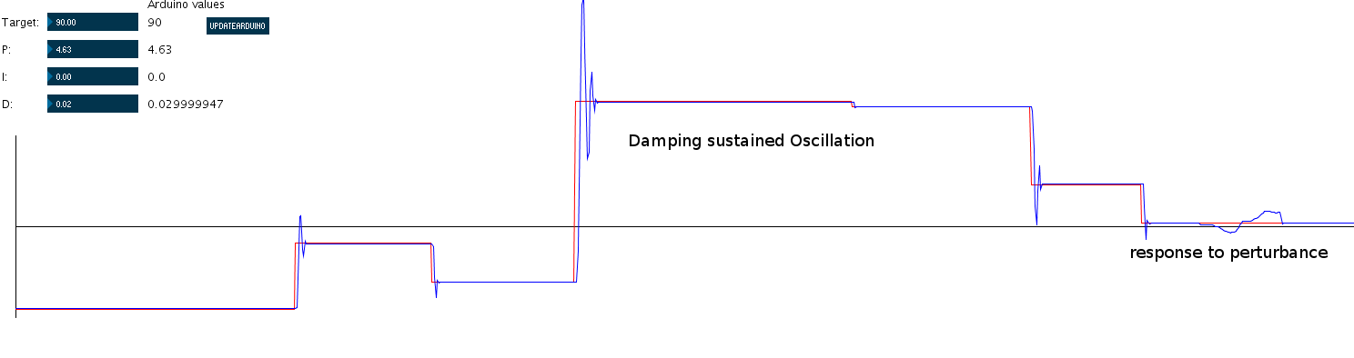 Fig 3. Low Derivative Gain Constant
Now, we introduce a small derivative gain constant Kd = 0.03. This derivative gain stabilizes the controller by damping the oscillation be decaying the amplitude of consecutive overshoot and undershoot. For small perturbances, this small gain is sufficient to stabilize the system.
Fig 3. Low Derivative Gain Constant
Now, we introduce a small derivative gain constant Kd = 0.03. This derivative gain stabilizes the controller by damping the oscillation be decaying the amplitude of consecutive overshoot and undershoot. For small perturbances, this small gain is sufficient to stabilize the system.
 Fig 4. High Derivative Gain Constant
If we increase the derivative gain to Kd = 0.81 [Note: This is numerically low value but the controller is highly sensitive to this value.], observe that the overshoot is gone. This system can be called critically damped if the transient time is suitable for a system. For systems that require lower transient time, this controllers would make the system overdamped. For our system, we observe a zitteriness (feel the twiddler shake and hear its noise. see it in video at the end of this page) at the end of the transient. This zitteriness suggests that, our system can come to the steady state faster by removing the zitter.
Also note that, for a high value of Kp and high value of Kd, the system does not oscillate at steady state and does not show any steady state error. Now, we understand that we can either increase the Kp term to bring the transient response time to low value and taking a chance on overshoot or decrease the Kd term to remove the zitter. Its also possible that we can increase the Kp gain to bring the transient response time to low value. If we observe any overshoot, we increase the Kd term. Fig 5-6 show the effects of changing those parameters.
Fig 4. High Derivative Gain Constant
If we increase the derivative gain to Kd = 0.81 [Note: This is numerically low value but the controller is highly sensitive to this value.], observe that the overshoot is gone. This system can be called critically damped if the transient time is suitable for a system. For systems that require lower transient time, this controllers would make the system overdamped. For our system, we observe a zitteriness (feel the twiddler shake and hear its noise. see it in video at the end of this page) at the end of the transient. This zitteriness suggests that, our system can come to the steady state faster by removing the zitter.
Also note that, for a high value of Kp and high value of Kd, the system does not oscillate at steady state and does not show any steady state error. Now, we understand that we can either increase the Kp term to bring the transient response time to low value and taking a chance on overshoot or decrease the Kd term to remove the zitter. Its also possible that we can increase the Kp gain to bring the transient response time to low value. If we observe any overshoot, we increase the Kd term. Fig 5-6 show the effects of changing those parameters.
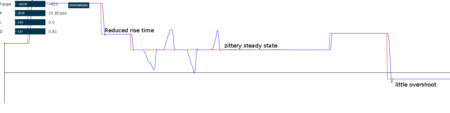 Fig 5. Tuning PD controller
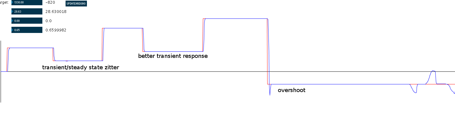 Fig 6. Tuned PD Controller
PI Controller
Integral gain is applied to the sum of error accumulated to over time. This gain is applied to systems that cannot reach its steady state value. In our example described above, the system was able to reach the steady state because it was strong enough to produce a momentum to bring the system to its new target state and damp enough to avoid oscillation. If the system was underactuated with low proportional gain we observed a steady state error as in Fig 1. In Fig 7, we increase the Kp term [Note: the figure shows the final value of Kp and Kd but we are describing how the graph evolves] to observe an oscillation that damps but still produces a steady state error. Now we add an integral gain Ki= 0.1. When we perturbe the system for sometime to let the error to accumulate on the integrator, it damps to slowly, ends with a steady state error. Now, the integral gain slowly corrects the position to final steady state. What if we increase the Ki gain to bring steady state faster. NO!!!. Because the integral gain is applied to cumulative error its value can easily reach the limiting value of the datatype being used to store the error. The effect of the integral term could easily make the system unstable. In this example, we introduce a sustained perturbance on an increased integral gain system with Ki=0.53, we observe the system go unstable. This instability can be attributed to slow reacting nature of the integrator gain and integrator winding up to datatype limitations.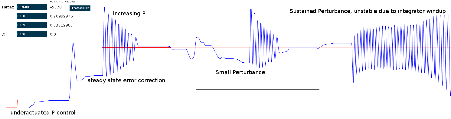 Fig 7. PI controller
PID Controller and other parameters
Now that we have observed the effects of proportional, integral and derivative gains of a system. Lets use all these parameters in our system. BAD IDEA!!! First, need to understand our system and if we need a PID controller or not. Currently, we are running our PID controller every milliseconds. Our system is able to tuned well in Fig 6 using a PD controller. We can say that, our system can be fairly stabilized using a linear controller like a PID with not integral gain. But, if our system was not linear, would a PID control be able to control the sytem? We observed our system going a little bouncy when we decreased the sampling rate to 100ms (i.e. PID controller runs ten times every second) of the PID control loop. When the sampling rate is decreased, the system has more time to respond and the controller has more time to observe the effects of its actions. This can make the system slow and also very sensitive to gains because all the observations are longer time leading to larger values of errors. With a Kp gain = 0.4 and a sampling time Ts = 100ms, we see in Fig 5. the system fails to keep track of its action and senses.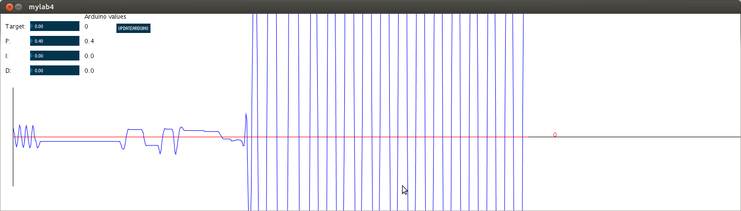 Fig 8. Slow responding system
So, we don't want a slow responding system. What if we could increase the response of the system by sampling as fast as we could? We are using Ts = 1ms. What if we decrease it to even lower value. May be could first check how long does our controller take to execute. We can do this observing the time difference between consecutive PID loop. We observe that the value is not always fixed. How??? An example situation can be that for each sensor input the system has to keep track of position of encoders. If the system is running fast, it would first have to respond to sensor signals slowing down the PID loop. We don't want to sample as fast as we could because the PID gains are sensitive to noise and our errors between different iterations of the PID could have different significance. So, we will have to use some technique to be consistent when we execute the PID control. Using Timer interrupt service routines can help make the system more stable by keeping the PID gains noise free.
In our system, we used default PID parameter of Ts = 1ms. Since PID loop would not take longer than 1ms, 1ms was the fastest that we could go. Beyond that, we were constrained by not only the system but also the processing speed. Hence, we observed more stable response using interrupt service routine versus the default system. We repeated the PID tuning as above to observe the differences (explanation beyond scope of this report).
Fig 8. Slow responding system
So, we don't want a slow responding system. What if we could increase the response of the system by sampling as fast as we could? We are using Ts = 1ms. What if we decrease it to even lower value. May be could first check how long does our controller take to execute. We can do this observing the time difference between consecutive PID loop. We observe that the value is not always fixed. How??? An example situation can be that for each sensor input the system has to keep track of position of encoders. If the system is running fast, it would first have to respond to sensor signals slowing down the PID loop. We don't want to sample as fast as we could because the PID gains are sensitive to noise and our errors between different iterations of the PID could have different significance. So, we will have to use some technique to be consistent when we execute the PID control. Using Timer interrupt service routines can help make the system more stable by keeping the PID gains noise free.
In our system, we used default PID parameter of Ts = 1ms. Since PID loop would not take longer than 1ms, 1ms was the fastest that we could go. Beyond that, we were constrained by not only the system but also the processing speed. Hence, we observed more stable response using interrupt service routine versus the default system. We repeated the PID tuning as above to observe the differences (explanation beyond scope of this report).
Implementation of Virtual Wall
We implement virtual wall as controller that operates on one side of the target position. We assume that the wall boundary is at position x = 0 and there is free space at x < 0. First we test our system using a single P controller. The proportional controller behaved like a spring as shown in Fig 9 and video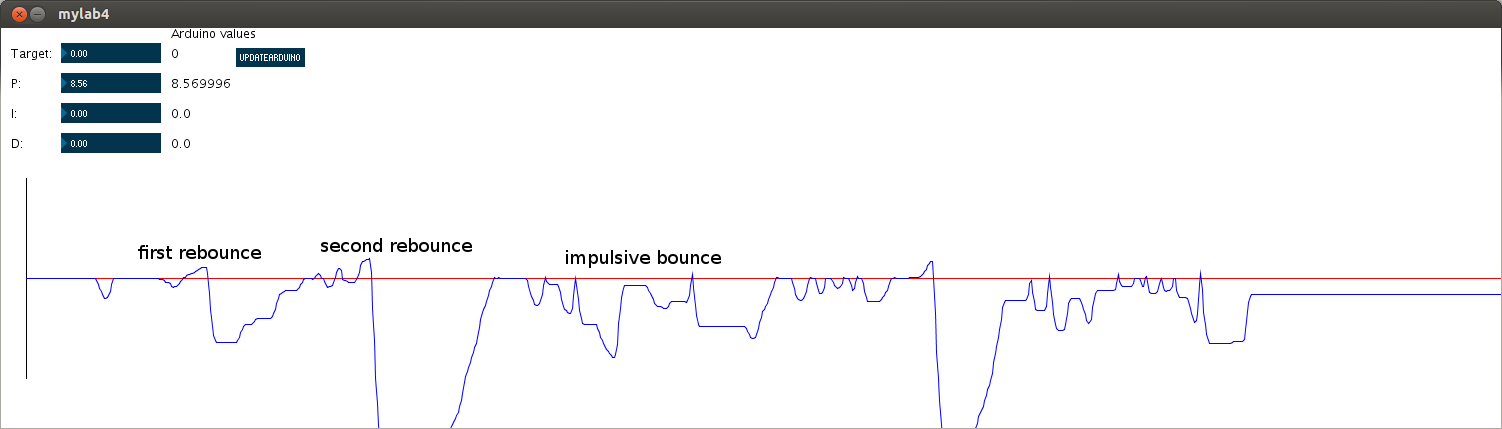 Fig 9. Spring Wall system video
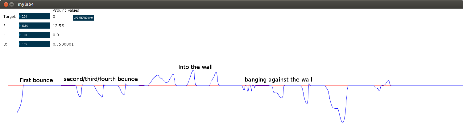 Fig 10. Stiffer Virtual Wall system video
Reflections
In this lab, we learnt about the effects of different gain terms in PID. I learnt that, each of these gain terms have different effects and we should understand if our system needs any or all of the gain terms in a PID control equation. My experimentation with PID control suggests that, we should keep the system overactuated to be able to have a robust control. Our Twiddler when not boosted by additional power supply could not produce enough torque to hold a loaded twiddler (it failed when my hand was on the twiddler). So, our system must have enough power to be able to move under loaded condition. Sampling as fast as possible is equally important as sampling at consistent time. Simulating a virtual wall was a good exercise of tuning a PID Controller. -- BikramAdhikari - 14 Mar 2014

| I | Attachment | History | Action | Size | Date | Who | Comment |
|---|---|---|---|---|---|---|---|
| |
100ms_overshoot.png | r1 | manage | 22.8 K | 2014-03-14 - 16:58 | BikramAdhikari | |
| |
PI_labeled.png | r1 | manage | 49.6 K | 2014-03-14 - 16:20 | BikramAdhikari | |
| |
Spring_wall_labeled.png | r1 | manage | 29.4 K | 2014-03-14 - 17:20 | BikramAdhikari | |
| |
Tunind_PD_better_labeled.png | r1 | manage | 18.0 K | 2014-03-14 - 15:46 | BikramAdhikari | |
| |
Tuning_PD_labeled.png | r1 | manage | 19.8 K | 2014-03-14 - 15:47 | BikramAdhikari | |
| |
Virtual_Wall_labeled.png | r1 | manage | 26.7 K | 2014-03-14 - 17:21 | BikramAdhikari | |
| |
high_D_labeled.png | r1 | manage | 19.4 K | 2014-03-14 - 15:35 | BikramAdhikari | |
| |
high_Dval_labeled.png | r1 | manage | 19.4 K | 2014-03-14 - 15:57 | BikramAdhikari | |
| |
high_P_labeled.png | r1 | manage | 49.0 K | 2014-03-14 - 15:15 | BikramAdhikari | |
| |
low_D_labeled.png | r1 | manage | 19.0 K | 2014-03-14 - 15:43 | BikramAdhikari | |
| |
low_Dval_labeled.png | r1 | manage | 19.0 K | 2014-03-14 - 15:45 | BikramAdhikari | |
| |
low_p_labeled.png | r1 | manage | 19.7 K | 2014-03-14 - 15:16 | BikramAdhikari |
Topic revision: r3 - 2014-03-14 - BikramAdhikari

Ideas, requests, problems regarding TWiki? Send feedback