Based on a rough empirical estimate, we will assume that the highest values of the node potentials for each of the stops is:
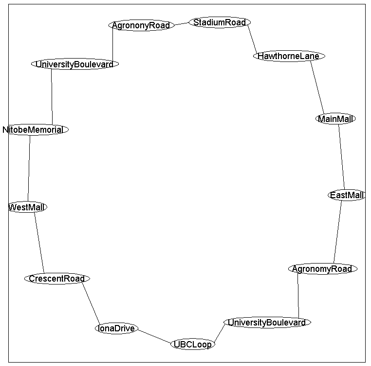
The bus makes 13 stops, and we will assume that at each stop we might have
between 0 and 24 people (the maximum capacity of the bus) waiting at it. Since the bus route forms a loop and their exists a dependency between the number of people waiting at
adjacent stops, we will use the following loop-structured graph:
Based on a rough empirical estimate, we will assume that the highest values of the node potentials for each of the
stops is:
| Stop | Highest nodePot |
| UBCLoop | 10 |
| UniversityBoulevard | 8 |
| AgronomyRoad | 0 |
| EastMall | 3 |
| MainMall | 5 |
| HawthorneLane | 4 |
| StadiumRoad | 0 |
| AgrononyRoad | 5 |
| UniversityBoulevard | 0 |
| NitobeMemorial | 0 |
| WestMall | 0 |
| CrescentRoad | 0 |
| IonaDrive | 0 |
To model correlations between adjacent stops, we will put the highest edge potential on adjacent stops having the same number of people. Subsequently, we will make the edge potentials decay according to a Gaussian based on the difference between the number of people at adjacent stops.
nNodes = 13;
nStates = 25;
adj = zeros(nNodes);
for i = 1:nNodes-1
    adj(i,i+1) = 1;
end
adj(nNodes,1) = 1;
adj = adj+adj';
edgeStruct = UGM_makeEdgeStruct(adj,nStates);
Now the node potentials:
busy = [10
    8
    0
    3
    5
    4
    0
    5
    0
    0
    0
    0
    0];
nodePot = zeros(nNodes,nStates);
for n = 1:nNodes
   for s = 1:nStates
      nodePot(n,s) = exp(-(1/10)*(busy(n)-(s-1))^2);
   end
end
And finally the edge potentials:
edgePot = zeros(nStates);
for s1 = 1:nStates
    for s2 = 1:nStates
        edgePot(s1,s2) = exp(-(1/100)*(s1-s2)^2);
    end
end
edgePot = repmat(edgePot,[1 1 edgeStruct.nEdges]);
clamped = zeros(nNodes,1);
clamped(1) = 11;
optimalDecoding = UGM_Decode_Conditional(nodePot,edgePot,edgeStruct,clamped,@UGM_Decode_Tree);
optimalNumber = optimalDecoding-1
optimalNumber =
10
8
1
3
5
4
1
4
0
0
0
0
1
[nodeBel,edgeBel,logZ] = UGM_Infer_Conditional(nodePot,edgePot,edgeStruct,clamped,@UGM_Infer_Tree);
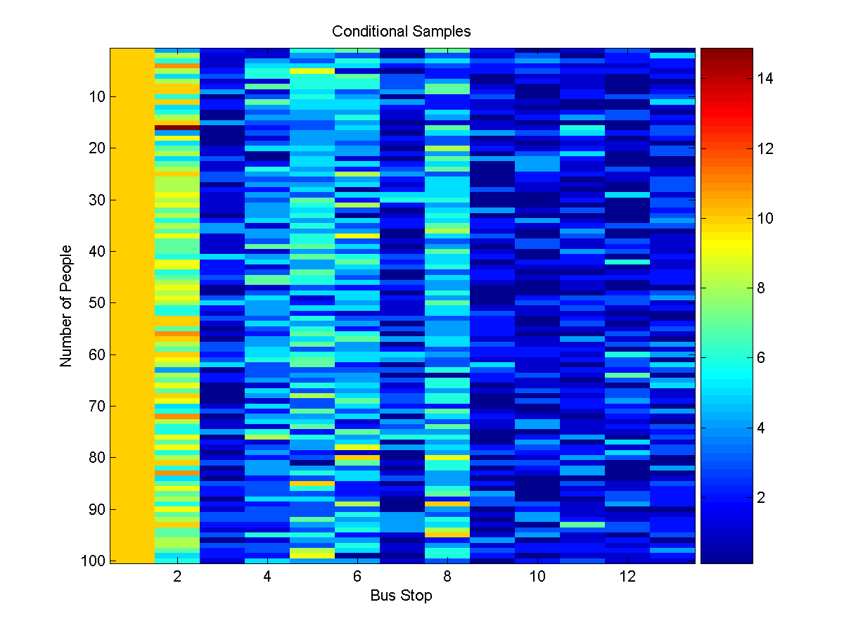
samples = UGM_Sample_Conditional(nodePot,edgePot,edgeStruct,clamped,@UGM_Sample_Tree);
figure(1);
imagesc(samples'-1);
xlabel('Bus Stop');
ylabel('Number of People');
title('Conditional Samples');
colorbar
We will use node 1 as the 'cutset', and use the cutset conditioning algorithm
to find the optimal decoding:
cutset = 1;
optimalDecoding = UGM_Decode_Cutset(nodePot,edgePot,edgeStruct,cutset)
optimalNumber2 = optimalDecoding-1;

optimalNumber =

     9
     8
     1
     3
     5
     4
     1
     4
     0
     0
     0
     0
     1
Cutset conditioning can also be used for computing the normalizing constant and
marginals. To compute the normalizing constant, we simply add up the
normalizing constants from the conditional UGMs (multiplied by the node and
edge potentials that are missing from the conditional UGM) under each possible
value(s) of the cutset variable(s). To compute marginals, we first compute conditional
marginals under each assignment to the cutset variables, and then normalize the
weighted sum of these marginals (where the weights come from the normalizing
constants of the conditional UGMs, together with the node and edge potentials
that are missing from the conditional UGM). This can be called with:
[nodeBel,edgeBel,logZ] = UGM_Infer_Cutset(nodePot,edgePot,edgeStruct,cutset);
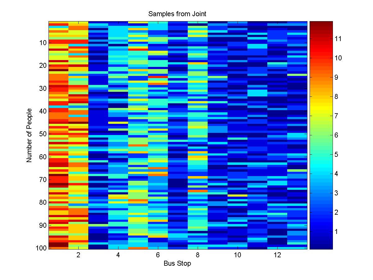
Sampling also works in an analogous way. We first compute the weights of the
different possible values of the cutset variables. Then we generate a random
value from the normalized distribution of the weights. This value is then used
to generate a sample of the remaining variables given the corresponding value
of the cutset variable. This can be called with:
samples = UGM_Sample_Cutset(nodePot,edgePot,edgeStruct,cutset);
figure(2);
imagesc(samples'-1);
xlabel('Bus Stop');
ylabel('Number of People');
title('Samples from Joint');
colorbar
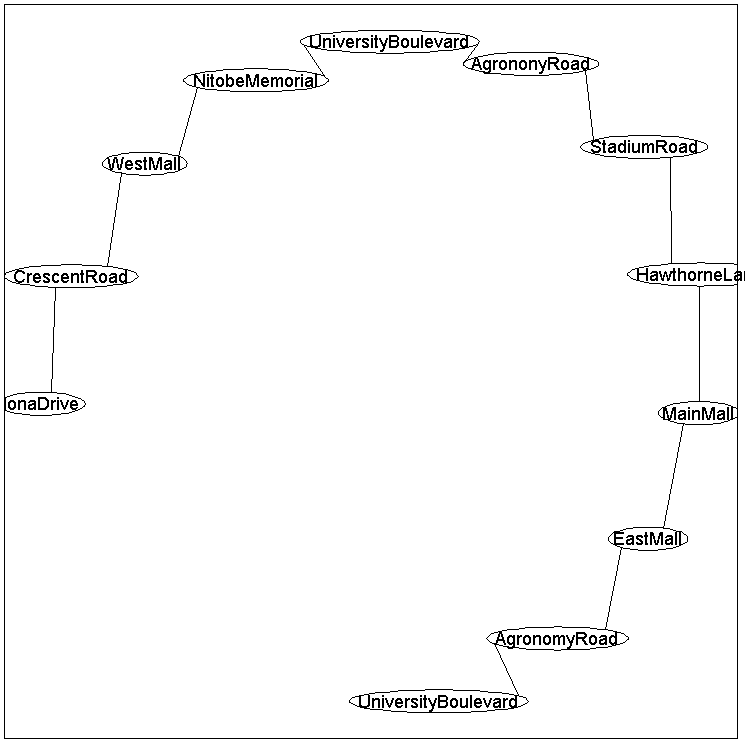
For example, consider a transit system with the following topological structure:
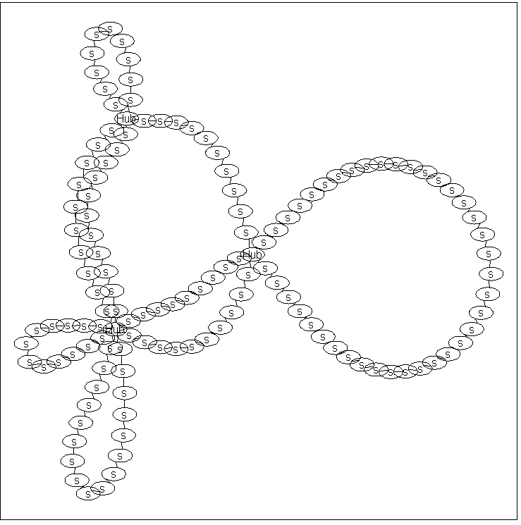
In this graph, there is no single node that we can condition on to make the
conditional graph structure a forest. This is because no single node can break
all of the loops present in the graph. However, if we simultaneously condition
on all three nodes labeled 'Hub', then the conditional UGM is a set of
independent chains. So, we can perform exact decoding/inference/sampling with
a cutset conditioning algorithm where we loop over all possible values of these
3 cutset nodes. In this graph, the 'Hub' variables are nodes 1;70;81, so we
can perform exact decoding/inference/sampling using:
cutset = [1 70 81];
optimalDecoding = UGM_Decode_Cutset(nodePot,edgePot,edgeStruct,cutset);
[nodeBel,edgeBel,logZ] = UGM_Infer_Cutset(nodePot,edgePot,edgeStruct,cutset);
samples = UGM_Sample_Cutset(nodePot,edgePot,edgeStruct,cutset);
Although it is efficient if the size of the cutset is small, in general the
runtime of cutset conditioning algorithms is exponential in the number of nodes
in the cutset (as well as the number of states). For example, if we want to
do decoding and the cutset needed to make the conditional UGM a forest has k
elements, we will need to do decoding in s^k forests
(where s is the number of states). Thus, cutset conditioning is only
practical when the graph structure allows us to find a small cutset.
In the model described above, the potentials on each edge
form Toeplitz
matrices.
In a forest-structured UGM with Toeplitz edge potentials, it is possible to
reduce the total computation time of the various belief propagation algorithms
from O(nNodes * nStates^2) down to O(nNodes * nStates * log(nStates)), by
taking advantage of techniques similar to the fast
Fourier transform. This improvement allows us to use
forest-structured models (or loopy models that admit a small cutset) where the number of states at each node is potentially
enormous. More efficient versions of belief propagation are also possible if our edge potenttial matrices do not have Toeplitz structure but have a different type of structure that allows us to multiply by the edge potential matrix in less than O(nStates^2). However, these types of speed-ups are not implemented in the current version of UGM.
PREVIOUS DEMO NEXT DEMO