Kalman filter toolbox for Matlab
Kalman filter toolbox for Matlab
Written by Kevin Murphy, 1998.
Last updated: 7 June 2004.
This toolbox supports filtering, smoothing and parameter estimation
(using EM) for Linear Dynamical Systems.
- kalman_filter
- kalman_smoother - implements the RTS equations
- learn_kalman - finds maximum likelihood estimates of the parameters using EM
- sample_lds - generate random samples
- AR_to_SS - convert Auto Regressive model of order k to State Space form
- SS_to_AR
- learn_AR - finds maximum likelihood estimates of the parameters
using least squares
For an excellent web site,
see
Welch/Bishop's KF
page.
For a brief intro, read on...
A Linear Dynamical System is a partially observed stochastic process with linear
dynamics and linear observations, both subject to Gaussian noise.
It can be defined as follows, where X(t) is the hidden state at time
t, and Y(t) is the observation.
   x(t+1) = F*x(t) + w(t),  w ~ N(0, Q),  x(0) ~ N(X(0), V(0))
   y(t)   = H*x(t) + v(t),  v ~ N(0, R)
The Kalman filter is an algorithm for performing filtering on this
model, i.e., computing P(X(t) | Y(1), ..., Y(t)).
The Rauch-Tung-Striebel (RTS) algorithm performs fixed-interval
offline smoothing, i.e., computing P(X(t) | Y(1), ..., Y(T)), for t <= T.
Here is a simple example.
Consider a particle moving in the plane at
constant velocity subject to random perturbations in its trajectory.
The new position (x1, x2) is the old position plus the velocity (dx1,
dx2) plus noise w.
[ x1(t)  ] =  [1 0 1 0] [ x1(t-1)  ] + [ wx1  ]
[ x2(t)  ]    [0 1 0 1] [ x2(t-1)  ]   [ wx2  ]
[ dx1(t) ]    [0 0 1 0] [ dx1(t-1) ]   [ wdx1 ]
[ dx2(t) ]    [0 0 0 1] [ dx2(t-1) ]   [ wdx2 ]
We assume we only observe the position of the particle.
[ y1(t) ] =  [1 0 0 0] [ x1(t)  ] + [ vx1 ]
[ y2(t) ]    [0 1 0 0] [ x2(t)  ]   [ vx2 ]
                       [ dx1(t) ]
                       [ dx2(t) ]
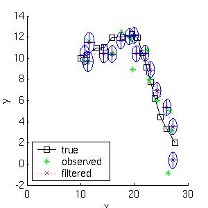
Suppose we start out at position (10,10) moving to the right with
velocity (1,0).
We sampled a random trajectory of length 15.
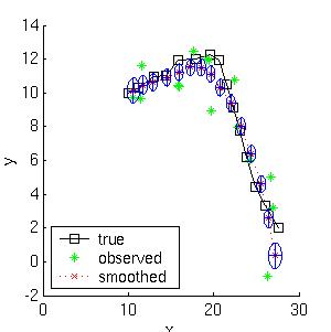
Below we show the filtered and smoothed trajectories.
The mean squared error of the filtered estimate is 4.9; for the
smoothed estimate it is 3.2.
Not only is the smoothed estimate better, but we know that
it is better, as illustrated by the smaller uncertainty ellipses;
this can help in e.g., data association problems.
Note how the smoothed ellipses are larger at the ends, because these
points have seen less data. Also, note how rapidly the filtered
ellipses reach their steady-state (Ricatti) values.
(Click here to see the code used to generate this
picture, which illustrates how easy it is to use the toolkit.)
For non-linear systems,
I highly recommend the
ReBEL
Matlab package,
which implements the extended Kalman filter,
the unscented Kalman filter, etc.
(See
Unscented filtering and nonlinear estimation,
S Julier and J Uhlmann, Proc. IEEE, 92(3), 401-422, 2004.
Also, a small
correction.)
For systems with non-Gaussian noise, I recommend
Particle
filtering (PF), which is a popular sequential Monte Carlo technique.
See
also this
discussion on
pros/cons of particle filters.
and the following tutorial:
M. Arulampalam, S. Maskell, N. Gordon, T. Clapp,
"A Tutorial on Particle
Filters for Online Nonlinear/Non-Gaussian Bayesian Tracking," IEEE
Transactions on Signal Processing, Volume 50, Number 2, February 2002, pp
174-189 (pdf cached here
The EKF can be used as a proposal distribution for a PF.
This method is better than either one alone.
The Unscented Particle Filter,
by R van der Merwe, A Doucet, JFG de Freitas and E Wan, May 2000.
Matlab software
for the UPF is also available.
Gatsby reading group on
nonlinear dynamical systems
-
Welch & Bishop,
Kalman filter web page,
the best place to start.
- T. Minka,
"From HMMs to LDSs",
tech report.
- T. Minka,
Bayesian inference in dynamic models -- an overview
, tech report, 2002
- K. Murphy.
"Filtering, Smoothing, and the Junction Tree Algorithm",.
tech. report, 1998.
- Roweis, S. and Ghahramani, Z. (1999)
A Unifying Review of Linear Gaussian Models
Neural Computation 11(2):305--345.
-
M. Arulampalam, S. Maskell, N. Gordon, T. Clapp,
"A Tutorial on Particle
Filters for Online Nonlinear/Non-Gaussian Bayesian Tracking," IEEE
Transactions on Signal Processing, Volume 50, Number 2, February 2002, pp
174-189.
- A. Doucet, N. de Freitas and N.J. Gordon,
"Sequential Monte Carlo Methods in Practice", Springer-Verlag, 2000