Michael DiBernardo (mddibern@cs.ubc.ca)
When an organism is infected by a virus, it will generate an immune response against it. The combination of the sloppy reproductive machinery of the virus and the selective pressure exerted by the immune system of the host will cause the virus to mutate, so that the sequence of the same virus will change across different hosts, and even across different tissues in the same host.
While many of the mutations sustained by the viral sequence are random, it is possible that a particular pattern of substitutions, insertions, and/or deletions may arise independently in several different viral instances. The prevalence of a pattern may indicate that it confers some advantage to the virus in a certain class of hosts; however, the pattern can also potentially be used by researchers to characterize new viral strains, and by drug developers as a target for therapy.
Recently, a subset or cohort of the African population that is immune to the HIV virus was discovered. These individuals are HIV-positive, but do not exhibit any of the symptoms of the infection or progress to being afflicted by full-blown AIDS. Much work is being done to characterize the differences between the genome sequences of the immune and susceptible populations.
Dr. Steven Jones and Dan Baluta of the BC Genome Sciences Center have decided to explore the situation from a different angle by studying the changes that the virus itself undergoes when it infects individuals from the susceptible and the immune populations. They have isolated viruses from several thousand HIV-immune and HIV-susceptible people and are in the process of sequencing all of these samples using high-thoroughput techniques. Dr. Jones plans to publish some preliminary results from the study in late November, and he expressed a desire for a single static overview of the sequence differences with respect to a canonical HIV viral sequence that could accompany the tabular data to be included in the publication. Dan Baluta has also indicated that he would like a tool that he could use to explore and interact with the data, although is not yet sure about what questions he hopes to answer through this interaction. He suggests that a visual overview of the data could stimulate the generation of such questions by identifying regions or patterns of interest.
Many software tools have been written to visualize biological features and differences across multiple sequences. However, there do not exist any such tools to visualize differences across more than a few hundred sequences, to my knowledge. Thus, our problem is largely one of scale: We wish to provide an overview of the sequence differences that provides enough detail to be useful without degenerating into clutter.
Visualization tools for biological sequence analysis are typically used to browse sequence alignments or sequence features. Alignment viewers are used to identify features that are shared among sequences for the purposes of generating an annotation, while a feature viewer is used to explore and modify a mature sequence annotation.
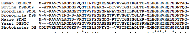
A sequence alignment can be viewed as a relation among two or more biological sequences that maps each nucleotide or amino acid in a sequence to a nucleotide or amino acid in all other sequences in the set. If one sequence contains a contiguous segment of nucleotides or amino acids that another does not, this difference can be interpreted as an insertion in the first sequence, or a deletion from the second sequence. The basic representation of a multiple sequence alignment across two or more genomes is a textual description of the alignment, as in Figure 1. Insertions/deletions, or indels, are identified by the use of a gap character, usually a '-'. Alignment viewers essentially take a textual alignment representation like the one in Figure 1 as input, and produce a visual representation or summary of the alignment.
A sequence feature is merely a region or attribute of interest in a particular sequence. Classes of sequence features include genes and intergenic regions, as well as GC-rich regions (blocks of sequence that have a relative abundance of guanine and cytosine nucleotides) and single-nucleotide polymorphisms (single nucleotide substitutions that are known to occur regularly in different instances of a particular species). Sequence features are often inferred by sequence alignment, and are the building blocks that biologists and bioinformaticians use to make inferences about the function of a sequence region.
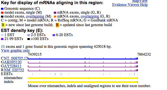
There are a variety of tools available to visualize sequence alignments, although many of them share common features. The NCBI MapViewer (Wheeler et al., 2002) serves as a browser for genome assemblies, which are essentially collections of alignments of sequence fragments used to infer the entire genome sequence. Of particular interest to this project is the Evidence Viewer (Figure 2) that identifies sequence features that have been inferred from alignments of known messenger RNAs to a genomic region. Sequences are represented as flatlines, and raised 'blips' in the lines are used to identify mismatches. The interface is rather bare-bones, and no overview is provided.
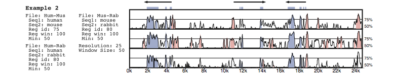
The VISTA alignment viewer (Mayor et al., 2000) is a more full-featured tool used specifically for processing raw alignments. A sliding window of a preset number of nucleotides is moved a nucleotide at a time over the alignment, and the percent identity of each sequence with respect to some 'base' sequence is computed in that window. This percent identity is then plotted as a line graph (Figure 3) so that one may quickly identify highly conserved and highly divergent regions. Colour is used to identify coding and intergenic regions. Although elegant, this approach does not scale to more than a handful of sequences. Also, sequences at the top and bottom of the display are more difficult to compare than those that are directly adjacent to one another.
Synplot (Gottgens et al., 2001) is another basic alignment viewer that relies on percent-identity plots (PIPs) to express sequence differences. However, Synplot also explicity represents insertions and deletions as gaps in the lines representing the first or second sequence, respectively. Colour is again used to highlight sequence features, although some spatial encoding is also used to emphasize coding regions (Figure 4).
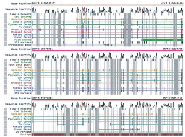
KBrowser (Chakrabarti and Pachter, 2004) is essentially a feature viewer that compares the features of multiple genomes simultaneously; however, alignment data (in the form of percent identity plots) are also displayed. KBrowser unfortunately lists all of the data tracks for a single genome in a continguous block, instead of interleaving the tracks for each genome (Figure 5). This makes it very difficult to compare specific sequence features to one another. Displaying indels as grey bands that stretch across all tracks is effective, but because substititutions are only shown across one track it appears as if they are less important than indels, which may or may not be the case depending on the problem being addressed.
ECRBrowser (Ovcharenko et al, 2004) is a multiple alignment viewer that seeks to emphasize evolutionarily conserved regions across vertebrate genomes, regardless of position or function. These regions are identified by shared peaks in PIP plots and are outlined with a box when detected by the software (Figure 6). Such an ECR can then be easily extracted and viewed in more detail. Making this particular operation a fast one is a good design decision, because the extraction of conserved sequence regions is almost always the purpose of a sequence analysis. A chromosomal overview is linked to the main view to maintain positional context, and features of sequence regions are again encoded with colour.
While the browsers that have been discussed thus far have their own individual strengths and weaknesses, they all share a common 'look and feel'. Sequences are displayed as lines, sequence features are displayed on surrounding lines or 'tracks', and percent-identity plots are used to display an overview of sequence similarity. While this homogenuity makes it moderately difficult to select one tool over another, it does suggest that there are certain types of displays that biologists are very familiar with when it comes to sequence analysis.
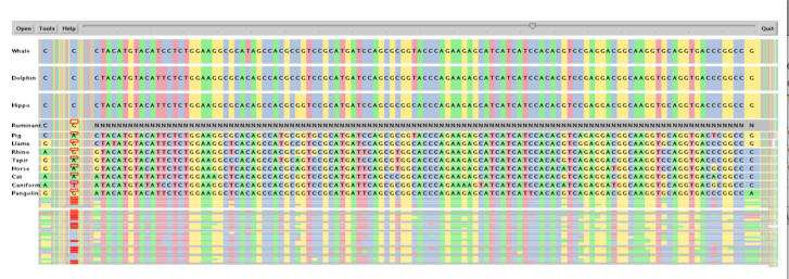
However, some alignment viewers have sought to break the mold. SequenceJuxtaposer (Munzner et al., 2004) uses an 'accordian drawing' rubber sheet metaphor to display a large number of sequences at one time while maintaining some overall context (Figure 7). Regions of interest can be identified across some number of sequences by drawing a box around them and 'stretching' them so that they are made larger with respect to their surroundings. Nucleotides are represented as colour-coded boxes, and when they are large enough in the display, their single-letter codes are rendered as text within the box. Indels are encoded as greyed-out boxes in the sequences that do not share the insertion. The rubber-sheet metaphor permits the display of a very large number of sequences at a very high resolution.
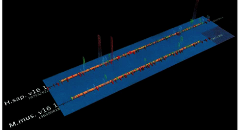
SockEye (Montgomery et al., 2004) is a 3D alignment viewer that differs from the 2D alignment viewers discussed thus far by using the third spatial dimension to encode the significance of the alignment at a given region (Figure 8). However, the perspective view makes it difficult to compare the thin vertical bar charts that represent the alignment quality, and the fact that they are rendered with transparency only amplifies this problem. No attempt is made to use the third dimension to alleviate the difficulty of having to lay sequences side-by-side for direct comparison; sequences at the top and bottom of the layout are still much more difficult to compare against each other than those that are directly adjacent.
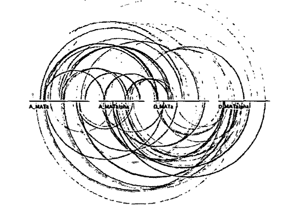
The biological arc diagram (Spell, Brady, and Dietrich, 2003), known as a BARD, was developed to reduce the difficulty of comparing sequences that are not laid out directly adjacent to one another. Arcs are drawn between aligned bases in line representations of the sequences that compose the alignment (Figure 9). However, this results in frequent line crossings that usually have little or no significance in the structure of the alignment, giving a general impression of visual clutter. Also, effective comparisons are still easier between adjacent sequences, because one does not have to follow the arcs as far.
Some researchers have also applied dimensionality reduction techniques to alignment display. For example, Tsalenko et al. were interested in classifying certain sequence divergences with respect to their ability to be used as markers for predisposition to diabetes (Tsalenko et al. 2003). Thus, instead of using a standard display method to identify potential divergent regions of interest, they instead enumerated all combinations of computationally identified sequence differences and tested the efficacy of each such combination when it was used as a marker for disease. For instance, if a particular collection of SNPs was found only in the diabetic population, one would strongly expect that an undiagnosed individual that also carries these SNPs in their genome sequence would be highly predisposed to diabetes. This concept was implemented as an assessment of 'information gain' for each combination of sequence differences, and a visualization of the information gain provided by each combination was used to select the best markers.
Feature viewers differ from alignment viewers in that they are more concerned with displaying the unique features of a sequence or a set of sequences than they are with displaying differences between the sequences in the set.
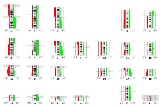
Caryoscope (Awad et al., 2004) and the Progenetix.net browser (Baudis and Cleary, 2001) are simple feature viewers that allow a high-level overview of an entire genome with respect to a single quantitative variate of interest. The genome is segmented into chromosomes, and coloured bar charts on each side of a chromosome indicate the value of the variate in the contained region (Figures 10, 11). Caryoscope allows the depiction of any sequence feature that can be described in a standard format known as GFF (General Feature Format); Progenetix.net displays the relative sequence loss and gain in tumour sequences with respect to the 'healthy' chromosomal sequence. Neither browser allows a more detailed view, apart from zooming in on an individual chromosome. I evaluated the freely-available Caryoscope software myself, and although it is elegant, the inability to provide more detail is frustrating, and performance degrades heavily when using even reasonably-sized datasets (such as those provided on the author's website).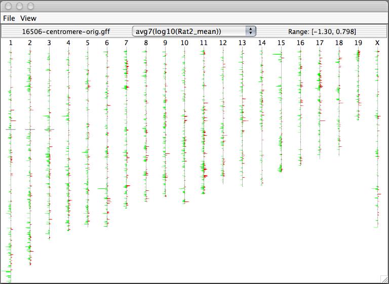
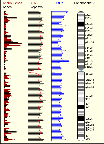
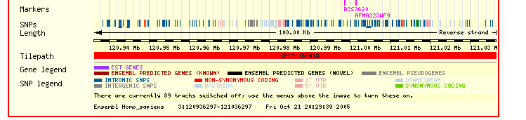
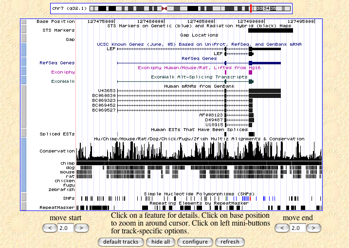
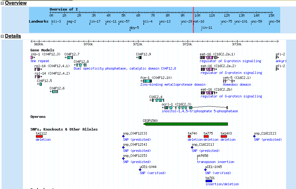
The ENSEMBL map viewer (Hubbard et al. 2005), the UCSC Genome Browser (Karolchik et al. 2003), and the open-source GBROWSE (Stein et al., 2002) are track-based feature viewers that share many similarities. All provide a chromosome-level overview of the genome being examined, and allow multiple levels of zoom in the secondary view (Figures 12, 13, 14). The user can add or remove feature tracks by manipulating a feature list. Glyphs on tracks are usually hyperlinked to specialized views: For instance, clicking on a glyph that represents a SNP will open a window that displays the list of known organisms that share the SNP, and any potential physiological differences that have been attributed with it. These viewers provide a great deal of detail that is easily interpreted for a small number of sequences (four or five on an average-sized display), largely because most of the data is spatially encoded. The disadvantage of these viewers is that they are delivered via dynamically generated HTML, and so any changes to a view require the page to be refreshed. Because most browsers will reorient the view at the very top of the page after a refresh, adding or removing a feature track will often require you to completely reorient your view before continuing with your work.
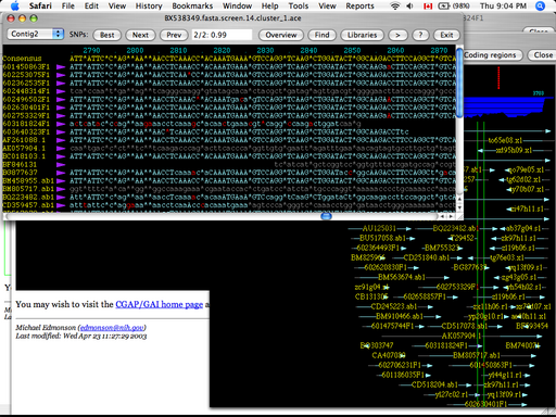
The SNP Launcher (Clifford et al. 2004) is a feature viewer that provides very detailed information about the quality of SNP assignments in a variety of genomes. All of the expressed sequence tag (EST) data that was used to infer the existence of a particular SNP is visualized spatially as a straight line beneath the canonical genome sequence. The relative amount of sequence evidence is depicted as a bar chart above the line that represents the genome. Clicking on a particular EST or genome region will open a window with a textual alignment view; unfortunately, there is no way to rearrange the order of the sequences presented in this detailed view. Further, SNPs in low- and high-covered regions are distinguished by the case of the character that represents the nucleotide, a difference that is difficult to pick out preattentively. SNPs in coding regions are coloured red, a common practice in many viewers, but the saturated red is hard to distinguish from the black background. There is no single overview that can be used as an entry point to the view depicted in Figure 15: One must specify a region of interest via a textual search query in an HTML form. Finally, the windows that are opened by the application are very difficult to close: A small square button in the lower-right of the window must be clicked, which is nonintuitive in almost any user interface.
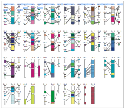
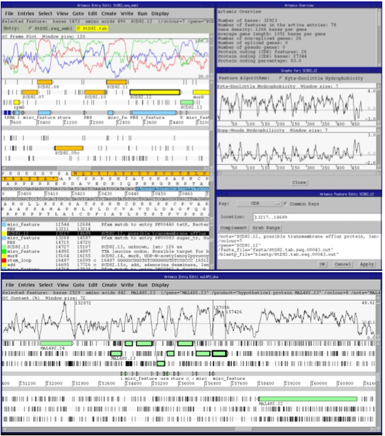
Artemis (Rutherford et al., 2000) and Apollo (Lewis et al., 2002) enable the user to access staggeringly detailed views of a single genome annotation. Apollo (Figure 16) provides more overviews than Artemis, such as depictions of high-level cross-chromosomal comparisons between vertebrate genomes (in this example, human and mouse), while Artemis provides a very detailed view that shows, among other things, all six open reading frames of the genome sequence at the region of interest, line-plots of GC content, hydrophobicity plots, and splicing and SNP patterns (Figure 17). In my (admittedly limited) experience working in genetics wet labs, this information is extremely useful when designing DNA sequence probes or primers that are to interact with the genomic region of interest, and so Artemis can get away with not providing any sort of overview; the intention is that it will only be invoked when a very specific region of interest has been identified.
There are essentially two audiences that will benefit from this project. The first audience is the HIV research community at large; In the publication that my clients (for lack of a better word) plan to submit this December, it will be necessary to communicate at a glance to HIV researchers whether the results affect their areas of research or not. A typical scenario would be a researcher that concentrates on the genes that code for coat proteins in HIV looking at the figure, and getting an instant idea as to whether there are a high proportion of SNPs in coat protein-coding genes in the immune cohort relative to the susceptible cohort. This researcher could then contact my clients for the sequence data specific to his gene of interest, and perform his own analyses from there.
The second audience is the set of researchers that are interested in examining the differences across the viral sequence as a whole. Dan Baluta falls into this category of researchers. It is hard for even he to specify what exactly his interaction with the data will entail until after we have produced a general overview to serve the needs of the first audience: However, one can imagine him using the overview to quickly get an idea of where the major divergences between immune and susceptible cohorts lie, and then exploring these divergent regions in more detail. For instance, if three genes are identified as having a large deletion frequency, one might then ask 'what is the subsequence that is, on average, being deleted?' If large scale insertions are observed, then one would likely want to know what the inserted sequence looks like: Is it consistently the same sequence, or is it random noise? (The first situation may indicate an addition of a functional group, while the latter may indicate that the insertion is disabling a gene.) Ideally, one would be able to then collect all of the mutant sequences that fit a certain difference pattern and explore them in detail.
I will present my proposed solution for the first problem first. We have already seen that biologists are accustomed to viewing certain types of information in specific ways (genomes as lines, frequencies as line or bar charts, etc), and because the visualization to address the first problem must be instantly interpretable and effective, I have decided that I must adhere to these conventions to the best of my ability. The solution will need to provide sufficient detail to allow experienced researchers to make an immediate judgment call on the experimental results, but must remain clear enough to allow fast interpretation.
Given these requirements, I decided on five variates that would have to be present in the visualization to make it useful:
Note that I need to display these variates (except for gene location) for both the susceptible and the immune cohorts, and so I am actually looking at nine variates. Also note that I have abstracted a multi-base deletions into multiple single-base deletions in order to avoid having to encode the length of the average deletion at after any given base. This is not so easy to do with insertions (at least, I could not think of a safe reduction in this case), and so I am forced to display two variates to describe them.
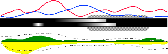
Figure 18 is a mockup of my proposed solution for the first problem. The canonical HIV genome sequence is represented as the thick black bar (with some gradienting that will be discussed in a moment) in the center of the display. Frequency of base substitution is displayed as a line graph overtop the genome 'bar', with the red line representing the immune cohort data and the blue line representing the susceptible cohort data. Frequency of base deletion is encoded as the lightness of the genome bar: The more frequent the deletion, the lighter the bar at that base. The top half of the bar will represent one of the cohorts, while the bottom half of the bar will represent the other. (This has been idealized as a smooth gradient in this diagram, but it the pattern exhibited by the experimental data will probably not be nearly as pretty.) The area/bar chart beneath the genome bar represents the frequency of insertion at a given base position, while the blitted lines plotted overtop represent the average length of those insertions. (Standard deviation from this average may also be a feasible quantity to display on this graph.) The texture of the blitted line prevents the generation of strong visual artifacts when it intersects with the area plots. Finally, regions of interest on the canonical sequence are surrounded with a greyscale rounded box, as in the right side of Figure 18.
The final overview will be composed of a series of these 'genome bar' displays stacked vertically atop one another. However, because the HIV genome is about 8 kilobases in length, it is entirely possible that I will have to represent more than one base with a single pixel. A simple average over the bases that share a pixel is not likely to be informative, so a sliding-window approach (such as that used in the PIP plots) may be used instead.
One can now see how someone would use such a diagram to address the first problem, which is essentially answering the question 'why should I care about this research?'. Our theoretical coat-protein researcher from the discussion above would look at this diagram and note that, while deletions in both cohorts tend to congregate around the left side of the depicted gene (from the bar gradients), and insertion frequencies and lengths are largely indistinguishable over the length of the gene (from the bottom plots), the immune cohort somehow exerts a much higher substitution rate in the gene than the susceptible cohort does (from the top plots).
Addressing the needs of the second audience is more difficult until we have some idea of what the actual experimental data looks like in the context of the described overview. My current plan is to link the overview shown in Figure 18 with a more detailed view where many pixels can be devoted to a single base, so that I can display such variates as the base-specific substitutions (ie how often does this A become a C, or a G, or a T?) and perhaps consensus sequences for the most common insertions and deletions that begin after each base. The overview will maintain context by drawing a box over the genomic region that is being explored in detail (such as in the UCSC and ENSEMBL browsers). However, until I receive more feedback from my clients, I do not want to spend too much time speculating at the nature of the secondary views. It is my hope that by presenting my mockups of the overview to Dan Baluta, I will generate some concrete criticisms that can be used both to improve the overview and to define features that would be useful in the secondary linked views.
I would like to implement this project from scratch or by building on a project that uses OpenGL, largely because it is the only graphics package that I am familiar with and I do not want to expend too much time learning the quirks of an equivalent technology. Because the approach I am taking is quite different from anything that has been done before in terms of biological sequence visualization, I do not expect to build on any existing genome/alignment viewers: However, I may refer to the code of the open source projects described in the Related Work section for hints on how to implement certain components of my overview. Portability is also a concern, because in all likelihood the viewer will be published over the web if the experiments are a success.
These criteria are causing me to gravitate towards using Java with OpenGL bindings, as was done with SequenceJuxtaposer. It would also likely be feasible to implement a version that can be cross-compiled over multiple platforms in C++, which would allow me in many cases to provide user interfaces more consistent with the environment provided by the user's operating system of choice. Development will be done on my Macintosh iBook laptop.
| Date | Work Completed |
|---|---|
| November 11 | Complete implementation of drafted overview using randomly-generated data and present to clients. |
| November 15 | Determine requirements for secondary views. Determine how revisions suggested by clients will be incorporated. |
| November 21 | Complete implementation of revisions suggested by clients from previous milestone. |
| December 2 | Completed implementation secondary views and additional features requested by clients. |
| December 5 | Collect revisions requested by clients based on Dec. 2nd release. |
| December 12 | Implementation completed (for purposes of this project). Begin project writeup and presentation preparation. |
| December 19 | Submit writeup and deliver final project presentation. |
My undergraduate degree was in bioinformatics, and I have worked through two research assistantships in sequence analysis and genome annotation. I do not have any direct experience in HIV genetics or large-scale sequencing studies, but I possess enough basic knowledge of molecular biology to understand the thrust of the study and the specific questions that Dr. Jones and Dan Baluta are interested in having answered.
Awad IA et al. Caryoscope: an Open Source Java application for viewing microarray data in a genomic context. BMC Bioinformatics, Oct.15;5:151, 2004.
Baudis M and Cleary ML. Progenetix.net: an online repository for molecular cytogenetic aberration data. Bioinformatics, 17(12):1228-9, 2001.
Chakrabarti K and Pachter L. Visualization of multiple genome annotations and alignments with the K-BROWSER. Genome Research, 14:716-720, 2004.
Clifford RJ et al. Bioinformatics tools for single nucleotide polymorphism discovery and analysis. Annals of the New York Academy of Science, 1020:101-9, 2004.
Gottgens B et al. Long-Range Comparison of Human and Mouse SCL Loci: Localized Regions of Sensitivity to Restriction Endonucleases Correspond Precisely with Peaks of Conserved Noncoding Sequences. Genome Research, 11(1):87-97, 2001.
Hubbard T et al. Ensembl 2005. Nucleic Acids Research, 33(Database issue):D447-53, 2005.
Karolchik D et al. The UCSC genome browser database. Nucleic Acids Research, 31(1):51-4, 2003.
Lewis SE et al. Apollo: a sequence annotation editor. Genome Biology, 3(12):RESEARCH0082 (Epub), 2002.
Mayor C et al. VISTA: Visualizing global DNA sequence alignments of arbitrary length. Bioinformatics, 16(11):1046-7, 2000.
Ovcharenko I et al. ECRBrowser: a tool for visualizing and accessing data from comparisons of multiple vertebrate genomes. Nucleic Acids Research, 32:W280-7, 2004.
Rutherford K et al. Artemis: Sequence visualization and annotation. Bioinformatics 16(10):944-5, 2000.
Slack J, Hildebrand K, Munzner T, and St. John, K. SequenceJuxtaposer: Fluid navigation for large-scale sequence comparison in context. Proceedings of the German Conference on Bioinformatics, 37-42, 2004.
Stein LD et al. The generic genome browser: a building block for a model organism system database. Genome Research, 12(10):1599-610, 2002.
Tsalenko A et al. Methods for analysis and visualization of SNP genotype data for complex diseases. Pacific Symposium on Biocomputing, 548-61, 2003.
Wheeler DL et al. Database resources of the National Center for Biotechnology Information: 2002 update. Nucleic Acids Research, 30(1):13-6, 2002.