Contents

% a simple demo of how to do structure learning with data from a DBN

Demo configuration

rand('seed',1); % Deterministic randomness
randn('seed',1);

HMM = 1;
HUSMEIER = 2;

dbnType = HMM;

Create a DBN

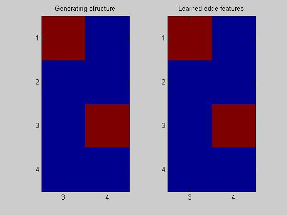
if dbnType == HMM

    % Build a "HMM" model, from which we will sample data
    % For the purposes of this demo, the HMM will be fully observed (BNSL cannot handle hidden variables)

    % Code that follows is from the BNT documentation
    intra = zeros(2);
    intra(1,2) = 1; % node 1 in slice t connects to node 2 in slice t

    inter = zeros(2);
    inter(1,1) = 1; % node 1 in slice t-1 connects to node 1 in slice t

    eclass1 = [1 2];
    eclass2 = [3 2];
    eclass = [eclass1 eclass2];

    Q = 2; % num hidden states
    O = 2; % num observable symbols

    % Original structure: (time flows to the right)
    % 2    4
    % ^    ^
    % 1 -> 3

    ns = [Q O];
    dnodes = 1:2;
    bnet = mk_dbn(intra, inter, ns, 'discrete', dnodes, 'eclass1', eclass1, 'eclass2', eclass2);
    prior0 = normalise(rand(Q,1));
    transmat0 = mk_stochastic(rand(Q,Q));
    obsmat0 = mk_stochastic(rand(Q,O));
    bnet.CPD{1} = tabular_CPD(bnet, 1, prior0);
    bnet.CPD{2} = tabular_CPD(bnet, 2, obsmat0);
    bnet.CPD{3} = tabular_CPD(bnet, 3, transmat0);

    maxFanIn = 3; % no fan-in constraint (nNodes-1)

    nData = 1000; % sample this many data

    % If the distribution is faithful, we should be able to learn (with an infinite sample size):
    % 2    4
    %      ^
    % 1 -> 3
    %
    % This is exactly what we hoped to learn (when represented as slices we only learn interior edges for the current
    % slice (ie. variables 3 & 4) and exterior edges from the past slice to the current slice).
    %
    % The edges are oriented by the layering (time) constraint.

end

Sample data from the DBN

data = cell2mat(sample_dbn(bnet, 'length', nData )); % sample some data from the DBN

Convert the data representation to one suitable for direct input into the BNSL routines

Transform the sampled data into a format suitable for BNSL (from time-series to time-slices) Returns a struct holding the new (doubled) # of nodes, a layering that encodes the flow of time, and the transformed data.

dataDbn = transformDbnData(data, 'maxFanIn', maxFanIn); % *** Important function

Learn the DBN back with the DP algorithm

Since all the parameters are randomly sampled, they could lead to a non-faithful distrubtion (ie. one that encodes conditionally independences not encoded by the DBN).

% These are the same functions used in simpleDemo.m (they are used throughout the BNSL package)
aflp = mkAllFamilyLogPrior( dataDbn.nNodes, 'nodeLayering', dataDbn.nodeLayering, 'maxFanIn', dataDbn.maxFanIn);
aflml = mkAllFamilyLogMargLik( dataDbn.data, 'nodeArity', bnet.node_sizes(:), 'impossibleFamilyMask', aflp~=-Inf, 'verbose', 1);
ep = computeAllEdgeProb( aflp, aflml);

% There is no point in doing structure learning on the first time step, since
% we cannot learn anything from a single data point (in terms of posterior features, such as edges)
% aflp = mkAllFamilyLogPrior( dataDbn.nNodes );
% aflml = mkAllFamilyLogMargLik( data(:,1), 'nodeArity', 2*ones(1,2));
% ep0 = computeAllEdgeProb( aflp, aflml);

Node 1/4
Node 2/4
Node 3/4
Node 4/4

Plot the result

nNodes = length(bnet.intra);
figure;
subplot(1,2,1); imagesc(bnet.dag(:,nNodes+1:end)); title('Generating structure'); axis('equal'); axis('tight');
set(gca,'ytick',1:dataDbn.nNodes); set(gca,'xtick',1:nNodes); set(gca,'xticklabel',nNodes+1:size(bnet.dag,2));

subplot(1,2,2); imagesc(ep(:,nNodes+1:end),[0 1]); title('Learned edge features'); axis('equal'); axis('tight');
set(gca,'ytick',1:dataDbn.nNodes); set(gca,'xtick',1:nNodes); set(gca,'xticklabel',nNodes+1:size(bnet.dag,2));

Published with MATLAB® 7.3