A Brief Introduction to Graphical Models and Bayesian Networks

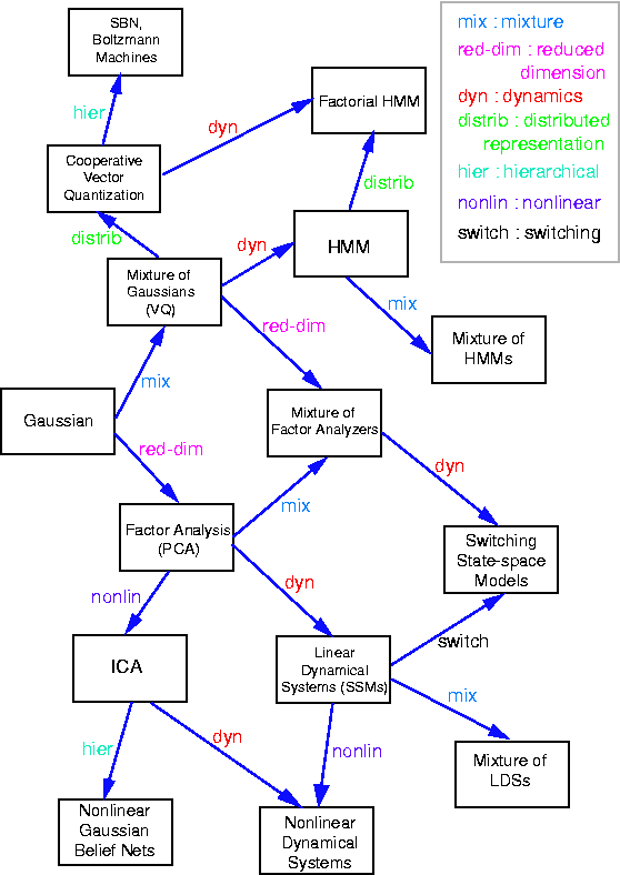
"Graphical models are a marriage between probability theory and graph theory. They provide a natural tool for dealing with two problems that occur throughout applied mathematics and engineering -- uncertainty and complexity -- and in particular they are playing an increasingly important role in the design and analysis of machine learning algorithms. Fundamental to the idea of a graphical model is the notion of modularity -- a complex system is built by combining simpler parts. Probability theory provides the glue whereby the parts are combined, ensuring that the system as a whole is consistent, and providing ways to interface models to data. The graph theoretic side of graphical models provides both an intuitively appealing interface by which humans can model highly-interacting sets of variables as well as a data structure that lends itself naturally to the design of efficient general-purpose algorithms.

Many of the classical multivariate probabalistic systems studied in fields such as statistics, systems engineering, information theory, pattern recognition and statistical mechanics are special cases of the general graphical model formalism -- examples include mixture models, factor analysis, hidden Markov models, Kalman filters and Ising models. The graphical model framework provides a way to view all of these systems as instances of a common underlying formalism. This view has many advantages -- in particular, specialized techniques that have been developed in one field can be transferred between research communities and exploited more widely. Moreover, the graphical model formalism provides a natural framework for the design of new systems." --- Michael Jordan, 1998.

We will briefly discuss the following topics.

• Representation, or, what exactly is a graphical model?
• Inference, or, how can we use these models to efficiently answer probabilistic queries?
• Learning, or, what do we do if we don't know what the model is?
• Decision theory, or, what happens when it is time to convert beliefs into actions?
• Applications, or, what's this all good for, anyway?

Representation

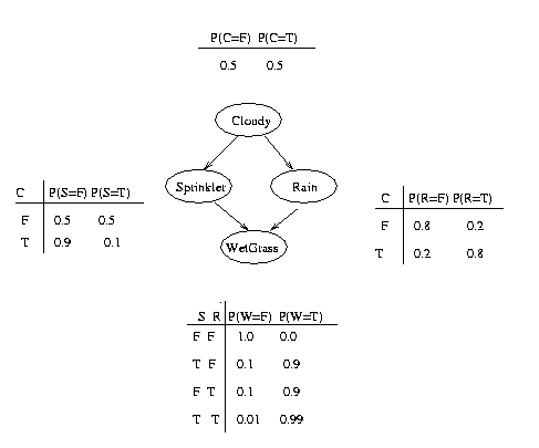
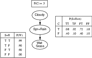
Consider the example above. Here, nodes represent binary random variables. We see that the event ``grass is wet'' (W=true) has two possible causes: either the water sprinker is on (S=true) or it is raining (R=true). The strength of this relationship is shown in the table below W; this is called W's conditional probability table (CPT). For example, we see that P(W=true | S=true, R=false) = 0.9 (second entry of second row), and hence, P(W=false | S=true, R=false) = 1 - 0.9 = 0.1, since each row must sum to one. Since the C node has no parents, its CPT specifies the prior probability that it is cloudy (in this case, 0.5).

The simplest statement of the conditional independence relationships encoded in a Bayesian network can be stated as follows: a node is independent of its ancestors given its parents, where the ancestor/parent relationship is with respect to some fixed topological ordering of the nodes. Let us see how we can use this fact to specify the joint distribution more compactly.

By the chain rule of probability, the joint probability of all the nodes in the graph above is

P(C, S, R, W) = P(C) * P(S|C) * P(R|C,S) * P(W|C,S,R)

P(C, S, R, W) = P(C) * P(S|C) * P(R|C) * P(W|S,R)

We can see that the conditional independence relationships allow us to represent the joint more compactly. Here the savings are minimal, but in general, if we had n binary nodes, the full joint would require O(2^n) parameters, but the factored form would only require O(n 2^k) parameters, where k is the maximum fan-in of a node.

We will now show how many popular statistical models can be represented as directed graphical models.

PCA, ICA, and all that

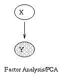
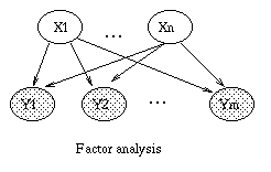
If we let the prior distribution on X be P(X=x) = N(x; 0, I), and the conditional distribution on Y be P(Y=y|X=x) = N(y; \mu + W x, \Psi), where \Psi is a diagonal matrix, then this model is called factor analysis. (The notation N(x; \mu, \Sigma) means the value of a Gaussian pdf with mean \mu and covariance \Sigma evaluated at the point (vector) x.) We usually assume that n \ll m, where X \in \real^n and Y \in \real^m, so the model is trying to explain a high dimensional vector as a linear combination of low dimensional features.

A common simplification is to assume isotropic noise, i.e., \Psi = \sigma I, for some scalar \sigma. In this case, the components of the vectors X and Y are uncorrelated, which we can explicitely represent using the model in Figure (b). It turns out that the maximum likelihood estimate of the factor loading matrix W in this case is given by the first m principle eigenvectors of the sample covariance matrix, with scalings determined by the eigenvalues and sigma. Classical PCA can be obtained by taking the \sigma \rightarrow 0 limit \cite{Tipping99,Roweis99}.

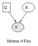
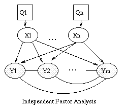
We can lift the restrictive assumption of linearity by modelling Y as a {\em mixture} of linear subspaces \cite{Tipping99}. This model is is shown in Figure~\ref{fig:mfa}(a). Q is a discrete latent (hidden) variable, that indicates which of the subspaces to use to generate Y. (In this tutorial, we adopt the (non-standard) convention notation that square nodes represent discrete random variables, and circles represent continuous random variables. We also use the (standard) convention that shaded nodes are observed, and clear nodes are (usually) hidden.) Mathematically, this can be written as

P(Q=i) &=& \pi_i \\
P(X=x) &=& N(x; 0, I) \\
P(Y=y|X=x,Q=i) &=& N(y; \mu_i + W_i x, \Psi_i)

Similarly, we can lift the restrictive assumption of Gaussian noise by modelling the prior on X as a mixture of Gaussians. One way to do this, known as independent factor analysis (IFA) \cite{Attias98}, is shown in Figure (b). (Technically, this is a chain graph: the undirected arcs between the components of Y indicate that they are correlated, i.e., that \Psi is not diagonal). This model is closely related to independent components analysis (ICA).

For more details, see the following papers.

• "EM algorithms for PCA and SPCA", Sam Roweis, NIPS 97.
• "Mixtures of probabilistic principal component analyzers", Tipping and Bishop, Neural Computation 11(2):443--482, 1999.
• Independent Factor Analysis, H. Attias, Neural Computation 11: 803--851, 1998.

HMMs, Kalman filters, and all that

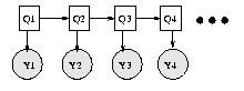
Consider the Bayesian network in Figure (a), which represents a hidden Markov model (HMM). This encodes the joint distribution

P(Q,Y) = P(Q_1) P(Y_1|Q_1) \prod_{t=2}^4 P(Q_t|Q_{t-1}) P(Y_t|Q_t) 

The Markov property states that the future is independent of the past given the present, i.e., Q_{t+1} \indep Q_{t-1} | Q_t. We can parameterize this Markov chain using a transition matrix, M_{ij} = P(Q_{t+1}=j | Q_t=i), and a prior distribution, \pi_i = P(Q_1 = i).

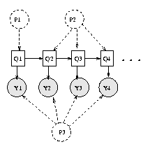
We have assumed that this is a homogeneous Markov chain, i.e., the parameters do not vary with time. This assumption can be made explicit by representing the parameters as nodes: see Figure(b): P1 represents \pi, P2 represents the transition matrix, and P3 represents the parameters for the observation model. If we think of these parameters as random variables (as in the Bayesian approach), parameter estimation becomes equivalent to inference. If we think of the parameters as fixed, but unknown, quantities, parameter estimation requires a separate learning procedure, to be discussed in Section~\ref{sec:learning}. In the latter case, we typically do not represent the parameters in the graph; shared parameters (as in this example) are implemented by specifying that the corresponding CPDs are ``tied''.

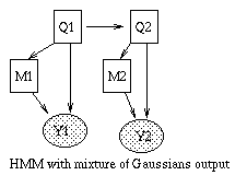
An HMM is a hidden Markov model because we don't see the states of the Markov chain, Q_t, but just a function of them, namely Y_t. For example, if Y_t is a vector, we might define P(Y_t=y|Q_t=i) = N(y; \mu_i, \Sigma_i). A richer model, widely used in speech recognition, is to model the output (conditioned on the hidden state) as a mixture of Gaussians. This is shown below.

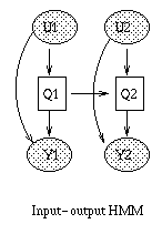
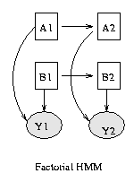
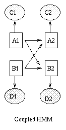
Some popular variations on the basic HMM theme are illustrated below (from left to right: an input-output HMM, a factorial HMM, a coupled HMM). (In the input-output model, the CPD P(Q|U) could be a softmax function, or a neural network.) If we have software to handle inference and learning in general Bayesian networks, all of these models becomes trivial to implement.

A linear dynamical system (LDS) has the same topology as the input-output HMM, except that the hidden nodes have linear-Gaussian CPDs. Replacing Q_t with X_t, the model becomes

P(X_1=x) &=& N(x; x_0, V_0) \\
P(X_{t+1}=x_{t+1}|U_t=u, X_t=x) &=& N(x_{t+1}; A x + B u, Q) \\
P(Y_t=y|X_t=x, U_t=u) &=& N(y; C x + D u, R) 

A generative model for generative models

• A Unifying Review of Linear Gaussian Models, Sam Roweis & Zoubin Ghahramani. Neural Computation 11(2) (1999) pp.305-345

Undirected graphical models

p(x) = \frac{1}{Z} \prod_{C \in {\cal C}} \psi_C(x_C)

Z = \sum_x \prod_{C \in {\cal C}} \psi_C(x_C).

P(x,y) \propto \Psi(x_1,x_2) \Psi(x_1,x_3) \Psi(x_2,x_4) \Psi(x_3,x_4)
  \prod_{i=1}^4 \Psi(x_i, y_i)

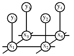
In the Ising model, the graph is a grid, so the cliques are edges, and the X_i nodes are binary. The potentials \Psi(x_i, x_j) for neighboring nodes i,j penalize differences: \Psi(x_i, x_j) = e^{-J(x_i,x_j)}, where J(x_i,x_j) = 1 if x_i=x_j and J(x_i,x_j) = -1 otherwise.

In low-level vision problems (e.g., \cite{Geman84,Freeman00c}), the X_i's are usually hidden, and each X_i node has its own ``private'' observation node Y_i, as in Figure~\ref{fig:vision_mrf}. The potential \Psi(x_i,y_i) = P(y_i|x_i) encodes the local likelihood; this is often a conditional Gaussian, where Y_i is the image intensity of pixel i, and X_i is the underlying (discrete) scene ``label''.

Inference

P(X|y) = \frac{P(y|X) P(X)}{P(y)}

             conditional likelihood * prior
posterior = ------------------------------
                   likelihood

where

is a normalizing constant, equal to the probability (likelihood) of the data. So we see that it is more likely that the grass is wet because it is raining: the likelihood ratio is 0.7079/0.4298 = 1.647.

In general, computing posterior esimates using Bayes' rule is computationally intractable. One way to see this is just to consider the normalizing constant, Z: in general, this involves a sum over an exponential number of terms. (For continuous random variables, the sum becomes an integral, which, except for certain notable cases like Gaussians, is not analytically tractable.) We will now see how we can use the conditional independence assumptions encoded in the graph to speed up exact inference.

Variable elimination

Notice that, as we perform the innermost sums, we create new terms, which need to be summed over in turn e.g.,

where

Continuing in this way,

where

This algorithm is called Variable Elimination. The principle of distributing sums over products can be generalized greatly to apply to any commutative semiring. This forms the basis of many common algorithms, such as Viterbi decoding and the Fast Fourier Transform. For details, see

• R. McEliece and S. M. Aji, 1998. "The Generalized Distributive Law", Submitted to IEEE Trans. Inform. Theory.

The amount of work we perform when computing a marginal is bounded by the size of the largest term that we encounter. Choosing a summation (elimination) ordering to minimize this is NP-hard, although greedy algorithms work well in practice.

Dynamic programming

For details, see

• "Probabilistic Reasoning in Intelligent Systems", Judea Pearl, 1988, 2nd ed.
• "Fusion and propogation with multiple observations in belief networks", Peot and Shachter, AI 48 (1991) p. 299-318.

Assuming for now that one is interested in exact inference, the most common approach is therefore to convert the graphical model into a tree, by clustering nodes together (see the example below, from \cite{Russell95}).

The need for approximate inference

Summary of approximate inference methods

• Sampling (Monte Carlo) methods. The simplest kind is importance sampling, where we draw random samples x from P(X), the (unconditional) distribution on the hidden variables, and then weight the samples by their likelihood, P(y|x), where y is the evidence. A more efficient approach in high dimensions is called Monte Carlo Markov Chain (MCMC), and includes as special cases Gibbs sampling and the Metropolis-Hastings algorithm. See e.g., \cite{Gilks96} for an introduction.

• Variational methods. The simplest example is the mean-field approximation, which exploits the law of large numbers to approximate large sums of random variables by their means. In particular, we essentially decouple all the nodes, and introduce a new parameter, called a variational parameter, for each node. We then iteratively update these variational parameters so as to minimize the cross-entropy (KL distance) between the approximate and true probability distributions. Updating the variational parameters becomes a proxy for inference. The mean-field approximation produces a lower bound on the likelihood. More sophisticated methods are possible, which give tighter lower (and upper) bounds. See \cite{Jordan98} for a tutorial.

• Loopy belief propagation. This entails applying Pearl's algorithm (see Section~\ref{sec:dynamic_programming}) to the original graph, even if it has loops (undirected cycles). This algorithm was inspired by the outstanding empirical success of turbo codes, which have been shown \cite{McEliece98b} to be an instance of this algorithm. Since then, further empirical work (e.g., \cite{Murphy99_loopy,Freeman00b}) has shown that the algorithm works well in other contexts, such as low-level vision. There has also been a lot of recent theoretical work analysing this algorithm \cite{Weiss99,Weiss00,Freeman00}, and figuring out the connections to other methods from statistical mechanics \cite{Yedidia00}.

Learning

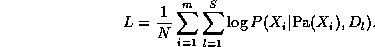
Structure   Observability    Method
---------------------------------------------
Known       Full             Maximum Likelihood Estimation
Known       Partial          EM (or gradient ascent)
Unknown     Full             Search through model space 
Unknown     Partial          EM + search through model space 

• W. L. Buntine, 1994. "Operations for Learning with Graphical Models", J. AI Research, 159--225.
• D. Heckerman, 1996. "A tutorial on learning with Bayesian networks", Microsoft Research tech. report, MSR-TR-95-06.

Known structure, full observability

\subsubsection{Directed graphical models} We assume that the goal of learning in this case is to find the maximum likelihood estimates (MLEs) of the parameters of each CPD, i.e., the parameter valyes which maximize the likelihood of the training data, which contains M cases (assumed to be independent). The normalized log-likelihood of the training set D = \{D_1, \ldots, D_M\} is a sum of terms, one for each node:

L = \frac{1}{M} \log \prod_{m=1}^M \Pr(D_m|G)
  = \frac{1}{M} \sum_{i=1}^{n} \sum_{m=1}^M \log P(X_i | Pa(X_i), D_m)

where Pa(X_i) are the parents of X_i. We see that the log-likelihood scoring function {\em decomposes} according to the structure of the graph, and hence we can maximize the contribution to the log-likelihood of each node independently. (It is simple to modify this to handle tied (shared) parameters.) If there are a small number of training cases compared to the number of parameters, we can use a prior to regularize the problem. In this case, we call the estimates maximum {\it a posterori} (MAP) estimates, as opposed to maximum likelihood estimates. In practice, this is not much harder computationally, as we will see below. For example, consider estimating the CPT for the W node in the water sprinkler example. If we have a set of training data, we can just count the number of times the grass is wet when it is raining and the sprinler is on, \#(W=1,S=1,R=1), the number of times the grass is wet when it is raining and the sprinkler is off, \#(W=1,S=0,R=1), etc. Given these counts (which are the sufficient statistics for a multinomial distribution), we can find the MLE of the CPT as follows:

\hat{P}_{ML}(W=w|S=s,R=r) = \frac{\#(W=w,S=s,R=r)}{\#(S=s,R=r)}

where the denominator is \#(S=s,R=r) = \#(W=0,S=s,R=r) + \#(W=1,S=s,R=r). Thus ``learning'' just amounts to counting (in the case of multinomial distributions). If a particular event is not seen in the training set, it will be assigned a probability of 0. To avoid this, we can use a Dirichlet prior; this just amounts to adding ``pseudo counts'' to the empirical counts. For example, using a uniform Dirichlet prior, the MAP estimate for the W node becomes

\hat{P}_{MAP}(W=w|S=s,R=r) = \frac{\#(W=w,S=s,R=r) + 1}{\#(S=s,R=r) + 2}

For Gaussian nodes, the MLE of the mean and covariance are the sample mean and covariance, and the MLE of the weight matrix is the least squares solution to the normal equations. For other kinds of CPDs (e.g., neural networks), more complex procedures are necessary for computing ML/MAP parameter estimates.

Undirected graphical models

The parameters of an undirected graphical model are the clique potentials. Maximum likelihood estimates of these can be computed using iterative proportional fitting (IPF) \cite{Jirousek95}.

Known structure, partial observability

\hat{P}(W=w|S=s,R=r) = E \#(W=w,S=s,R=r) / E \#(S=s,R=r)

E \#(e) = E \sum_m I(e | D_m) = \sum_m P(e | D_m)

Unknown structure, full observability

\Pr(G|D) = \frac{\Pr(D|G) \Pr(G)} {\Pr(D)}

L = \log \Pr(G|D) = \log \Pr(D|G) + \log \Pr(G) + c

P(D|G) = \int P(D|G,\theta) P(\theta|G) d \theta,

P(D|G) = \prod_{i=1}^n \int P(X_i | Pa(X_i), \theta_i) P(\theta_i) d \theta_i

Unknown structure, partial observability

Finally, we come to the hardest case of all, where the structure is unknown and there are hidden variables and/or missing data. The problem is that the marginal likelihood is intractable, requiring that we sum out all the latent variables Z as well as integrate out all the parameters \theta:

P(X|G) = \sum_{Z} \int P(X,Z|G,\theta) P(\theta|G) d \theta

This score does not decompose into a product of local terms. One approach is to use a Laplace approximation to the posterior of the parameters \cite{Chickering97}. After some algebra \cite{Heckerman98}, this leads to the following expression:

\log \Pr(D|G) \approx \log \Pr(D| G, \hat{\theta}_G) -  \frac{d}{2} \log M

where M is the number of samples, \hat{\theta}_G is the ML estimate of the parameters (computed using EM) and d is the dimension of the model. (In the fully observable case, the dimension of a model is the number of free parameters. In a model with hidden variables, it might be less than this.) This is called the Bayesian Information Criterion (BIC), and is equivalent to the Minimum Description Length (MDL) approach. The first term is just the likelihood and the second term is a penalty for model complexity. (Note that the BIC score is independent of the parameter prior.) Although the BIC score decomposes, local search algorithms (e.g., hill climbing) are still expensive, because we need to run EM at each step to compute \hat{\theta}. An alternative approach is to do the local search steps inside of the M step of EM --- this is called Structural EM, and provably converges to a local maximum of the BIC score \cite{Friedman97}.

Inventing new hidden nodes

So far, structure learning has meant finding the right connectivity between pre-existing nodes. A more challenging problem is inventing hidden nodes on demand. Hidden nodes can make a model much more compact, as we see the example above: If H is binary and the other nodes are trinary, and we assume full CPTs, the first network has 45 independent parameters, and the second has 708, even though they encode the same joint distribution.

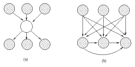
The standard approach is to keep adding hidden nodes one at a time, performing structure learning at each step, until the score drops. There has been some recent work on more intelligent heuristics. For example, dense clique-like graphs (such as that in Figure~\ref{fig:hidden_node}(b)) suggest that a hidden node should be added \cite{Elidan00}.

Decision Theory

In general, finding good controllers for non-linear, partially observed systems, usually with unknown parameters, is extremely challenging. One approach that shows some promise is reinforcement learning. Most of the work has been on systems which are fully observed (e.g., \cite{Sutton98}), but there has been some work on partially observed systems (e.g., \cite{Kaelbling98}). Recent policy search methods (e.g., \cite{Ng00}) show particular promise.

Applications

Special cases of Bayes nets were independently invented by many different communities many years ago, e.g., genetics (linkage analysis), speech recognition (HMMs), tracking (Kalman fitering), data compression (density estimation), channel coding (turbocodes), etc.

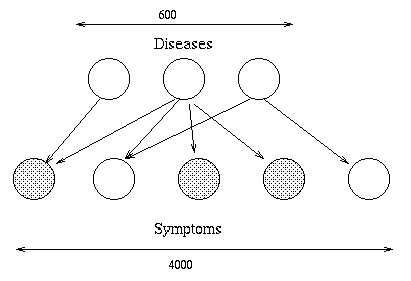
The general framework was developed by Pearl \cite{Pearl88} and various European researchers \cite{Jensen90,Cowell99}, who used it to make probabilistic expert systems. Many of these systems were used for medical diagnosis. A famous example is QMR-DT, a decision-theoretic reformulation of the Quick Medical Reference (QMR) model.

Here, the top layer represents hidden disease nodes, and the bottom layer represents observed symptom nodes. The goal is to infer the posterior probability of each disease given all the symptoms (which can be present, absent or unknown). QMR-DT is so densely connected that exact inference is impossible. Various approximation methods have been used, including sampling, variational and loopy belief propagation.

The same kind of diagnosis technology has since been widely adopted by Microsoft, e.g., the Answer Wizard of Office 95, the Office Assistant (the bouncy paperclip guy) of Office 97, and over 30 technical support troubleshooters. In fact, Microsoft now offers a Bayesian network API for Windows developers.

Another interesting fielded application is the Vista system, developed by Eric Horvitz. The Vista system is a decision-theoretic system that has been used at NASA Mission Control Center in Houston for several years. The system uses Bayesian networks to interpret live telemetry and provides advice on the likelihood of alternative failures of the space shuttle's propulsion systems. It also considers time criticality and recommends actions of the highest expected utility. The Vista system also employs decision-theoretic methods for controlling the display of information to dynamically identify the most important information to highlight. Horvitz has gone on to attempt to apply similar technology to Microsoft products, e.g., the Lumiere user interface project \cite{Horvitz98}.

For examples of other applications, see the special issue on UAI of Proc. ACM 38(3), 1995.

Recommended introductory reading

• Books
  • R. G. Cowell, A. P. Dawid, S. L. Lauritzen and D. J. Spiegelhalter, 1999. "Probabilistic Networks and Expert Systems". Springer-Verlag.
  • M. I. Jordan (ed), 1998. "Learning in Graphical Models", MIT Press.
• Review articles
  • P. Smyth, 1998. "Belief networks, hidden Markov models, and Markov random fields: a unifying view", Pattern Recognition Letters.
  • E. Charniak, 1991. "Bayesian Networks without Tears", AI magazine.
  • Sam Roweis & Zoubin Ghahramani, 1999. A Unifying Review of Linear Gaussian Models. Neural Computation 11(2) (1999) pp.305-345
• Exact Inference
  • C. Huang and A. Darwiche, 1996. "Inference in Belief Networks: A procedural guide", Intl. J. Approximate Reasoning, 15(3):225-263.
  • R. McEliece and S. M. Aji, 1998. "The Generalized Distributive Law", Submitted to IEEE Trans. Inform. Theory.
  • M. Peot and R. Shachter, 1991. "Fusion and propogation with multiple observations in belief networks", Artificial Intelligence, 48:299-318.
• Approximate Inference
  • M. I. Jordan, Z. Ghahramani, T. S. Jaakkola, and L. K. Saul, 1997. "An introduction to variational methods for graphical models."
  • D. MacKay, 1998. "An introduction to Monte Carlo methods".
  • T. Jaakkola and M. Jordan, 1998. "Variational probabilistic inference and the QMR-DT database"
• Learning
  • W. L. Buntine, 1994. "Operations for Learning with Graphical Models", J. AI Research, 159--225.
  • D. Heckerman, 1996. "A tutorial on learning with Bayesian networks", Microsoft Research tech. report, MSR-TR-95-06.
• DBNs
  • L. R. Rabiner, 1989. "A Tutorial in Hidden Markov Models and Selected Applications in Speech Recognition", Proc. of the IEEE, 77(2):257--286.
  • Z. Ghahramani, 1998. Learning Dynamic Bayesian Networks In C.L. Giles and M. Gori (eds.), Adaptive Processing of Sequences and Data Structures . Lecture Notes in Artificial Intelligence, 168-197. Berlin: Springer-Verlag.