 For a non-technical introduction, read
this LA times article
(10/28/96)
or this
Computer Shopper article (8/97).
For a brief technical introduction, see below.
For the gory details,
see the AUAI homepage
(Association for Uncertainty in Artificial Intelligence), or my list
of recommended reading at the end.
The UAI mailing list
is now archived and provides up-to-date information.
(See here for
the old UAI archive.)
I also maintain a list of Bayes Net software
packages, including my own Bayes Net
Toolbox for Matlab 5.
For a non-technical introduction, read
this LA times article
(10/28/96)
or this
Computer Shopper article (8/97).
For a brief technical introduction, see below.
For the gory details,
see the AUAI homepage
(Association for Uncertainty in Artificial Intelligence), or my list
of recommended reading at the end.
The UAI mailing list
is now archived and provides up-to-date information.
(See here for
the old UAI archive.)
I also maintain a list of Bayes Net software
packages, including my own Bayes Net
Toolbox for Matlab 5.
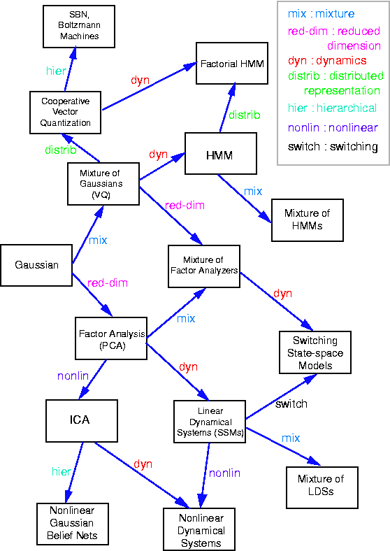
"Graphical models are a marriage of between probability theory and
graph theory. They provide a natural tool for dealing with two problems
that occur throughout applied mathematics and engineering --
uncertainty and complexity -- and in particular they are playing an
increasingly important role in the design and analysis of machine
learning algorithms. Fundamental to the idea of a graphical model is
the notion of modularity -- a complex system is built by combining
simpler parts. Probability theory provides the glue whereby the parts
are combined, ensuring that the system as a whole is consistent, and
providing ways to interface models to data. The graph theoretic side
of graphical models provides both an intuitively appealing interface
by which humans can model highly-interacting sets of variables as well
as a data structure that lends itself naturally to the design of
efficient general-purpose algorithms.
Many of the classical multivariate probabalistic systems studied in
fields such as statistics, systems engineering, information theory,
pattern recognition and statistical mechanics are special cases of the
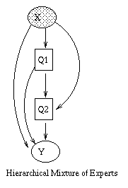
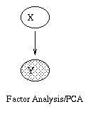
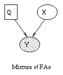
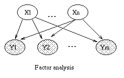
general graphical model formalism -- examples include mixture models,
factor analysis, hidden Markov models, Kalman filters and Ising
models. The graphical model framework provides a way to view all of
these systems as instances of a common underlying formalism. This view
has many advantages -- in particular, specialized techniques that have
been developed in one field can be transferred between research
communities and exploited more widely. Moreover, the graphical model
formalism provides a natural framework for the design of new systems."
We will briefly discuss the following topics.
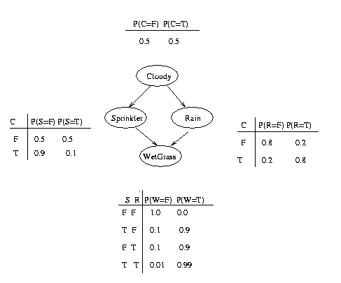
In addition to the graph structure, it is necessary to specify the parameters of the model. For an undirected model, we must specify a "potential function" for each clique in the graph. For a BN, we must specify the Conditional Probability Distribution (CPD) at each node. If the variables are discrete, this can be represented as a table (CPT), which lists the probability that the child node takes on each of its different values for each combination of values of its parents. Consider the following example, in which all nodes are binary, i.e., have two possible values, which we will denote by T (true) and F (false).
We see that the event "grass is wet" (W=true) has two possible causes: either the water sprinker is on (S=true) or it is raining (R=true). The strength of this relationship is shown in the table. For example, we see that Pr(W=true | S=true, R=false) = 0.9 (second row), and hence, Pr(W=false | S=true, R=false) = 1 - 0.9 = 0.1, since each row must sum to one. Since the C node has no parents, its CPT specifies the prior probability that it is cloudy (in this case, 0.5).
The simplest conditional independence relationship encoded in a Bayesian network can be stated as follows: a node is independent of its ancestors given its parents, where the ancestor/parent relationship is with respect to some fixed topological ordering of the nodes.
By the chain rule of probability, the joint probability of all the nodes in the graph above is
P(C, S, R, W) = P(C) * P(S|C) * P(R|C,S) * P(W|C,S,R)By using conditional independence relationships, we can rewrite this as
P(C, S, R, W) = P(C) * P(S|C) * P(R|C) * P(W|S,R)where we were allowed to simplify the third term because R is independent of S given its parent C, and the last term because W is independent of C given its parents S and R.
We can see that the conditional independence relationships allow us to represent the joint more compactly. Here the savings are minimal, but in general, if we had n binary nodes, the full joint would require O(2^n) space to represent, but the factored form would require O(n 2^k) space to represent, where k is the maximum fan-in of a node. And fewer parameters makes learning easier.


where

is a normalizing constant, equal to the probability (likelihood) of
the data.
So we see that it is more likely that the grass is wet because
it is raining:
the likelihood ratio is 0.7079/0.4298 = 1.647.
Notice that the two causes "compete" to "explain" the observed data. Hence S and R become conditionally dependent given that their common child, W, is observed, even though they are marginally independent. For example, suppose the grass is wet, but that we also know that it is raining. Then the posterior probability that the sprinkler is on goes down:
Pr(S=1|W=1,R=1) = 0.1945This is called "explaining away". In statistics, this is known as Berkson's paradox, or "selection bias". For a dramatic example of this effect, consider a college which admits students who are either brainy or sporty (or both!). Let C denote the event that someone is admitted to college, which is made true if they are either brainy (B) or sporty (S). Suppose in the general population, B and S are independent. We can model our conditional independence assumptions using a graph which is a V structure, with arrows pointing down:
   B   S
    \ /
     v
     C
Now look at a population of college students (those for which C is
observed to be true).
It will be found that being brainy makes you less likely to be sporty
and vice versa, because either property alone is sufficient to explain
the evidence on C.
In the water sprinkler example, we had evidence of an effect (wet grass), and inferred the most likely cause. This is called diagnostic, or "bottom up", reasoning, since it goes from effects to causes; it is a common task in expert systems. Bayes nets can also be used for causal, or "top down", reasoning. For example, we can compute the probability that the grass will be wet given that it is cloudy. Hence Bayes nets are often called "generative" models.
The above example showed what Bayes nets can be used for. Unfortunately, the method of first computing the full joint probability distribution, and then marginalizing out the unwanted nodes, takes time which is exponential in the number of nodes. As we will see later, the key to efficient inference is to exploit the factored form of the joint, i.e., the conditional independence properties of the model. So first we study such properties in a graph-theoretic way, and then return the numerical computations in the next section.
However, we can use the factored representation of the JPD to do this more efficiently. The key idea is to "push sums in" as far as possible when summing (marginalizing) out irrelevant terms, e.g.,
Notice that, as we perform the innermost sums, we create new terms, which need to be summed over in turn e.g.,

where

Continuing in this way,

where

This algorithm is called Variable Elimination. The principle of distributing sums over products can be generalized greatly to apply to any commutative semiring. This forms the basis of many common algorithms, such as Viterbi decoding and the Fast Fourier Transform. For details, see
The amount of work we perform when computing a marginal is bounded by the size of the largest term that we encounter. Choosing a summation (elimination) ordering to minimize this is NP-hard, although greedy algorithms work well in practice.
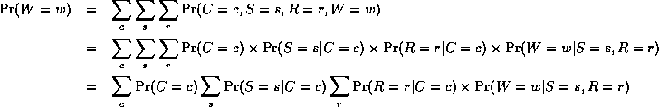
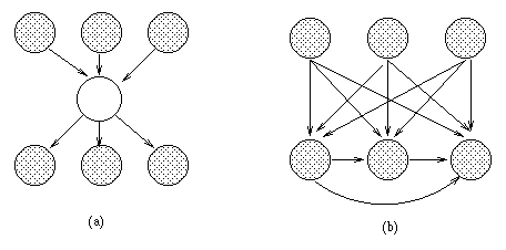
The most interesting case is the first column, when we have two arrows converging on a node X (so X is a "leaf" with two parents). If X is hidden, its parents are marginally independent, and hence the ball does not pass through (the ball being "turned around" is indicated by the curved arrows); but if X is observed, the parents become dependent, and the ball does pass through, because of the explaining away phenomenon. Notice that, if this graph was undirected, the child would always separate the parents; hence when converting a directed graph to an undirected graph, we must add links between "unmarried" parents who share a common child (i.e., "moralize" the graph) to prevent us reading off incorrect independence statements.
Now consider the second column in which we have two diverging arrows from X (so X is a "root"). If X is hidden, the children are dependent, because they have a hidden common cause, so the ball passes through. If X is observed, its children are rendered conditionally independent, so the ball does not pass through. Finally, consider the case in which we have one incoming and outgoing arrow to X. It is intuitive that the nodes upstream and downstream of X are dependent iff X is hidden, because conditioning on a node breaks the graph at that point.
Undirected graphical models are more popular with the physics and vision communities, and directed models are more popular with the AI and statistics communities. (It is possible to have a model with both directed and undirected arcs, which is called a chain graph.) For a careful study of the relationship between directed and undirected graphical models, see the books by Pearl88, Whittaker90, and Lauritzen96.
| 
|
| 
| 
| 
|
|  
|
|  
|
| 
| 
| 
|
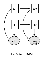
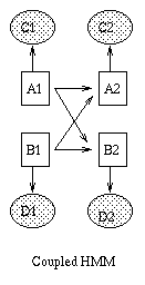
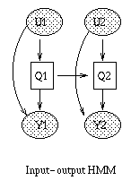
It is also possible to create temporal models with much more complicated topologies. See for example the BAT network, created here at Berkeley for monitoring freeway traffic.
When some of the observed nodes are thought of as inputs (actions), and some as outputs (percepts), the DBN becomes a POMDP. See also the section on decision theory below.
If the BN has undirected cycles (as in the water sprinkler example), local message passing algorithms run the risk of double counting. e.g., the information from S and R flowing into W is not independent, because it came from a common cause, C. The most common approach is therefore to convert the BN into a tree, by clustering nodes together, to form what is called a junction tree, and then running a local message passing algorithm on this tree. The message passing scheme could be Pearl's algorithm, but it is more common to use a variant designed for undirected models. For more details, click here
Structure   Observability    Method
---------------------------------------------
Known       Full             Maximum Likelihood Estimation
Known       Partial          EM (or gradient ascent)
Unknown     Full             Search through model space
Unknown     Partial          EM + search through model space
Consider estimating the Conditional Probability Table for the W node. If we have a set of training data, we can just count the number of times the grass is wet when it is raining and the sprinler is on, N(W=1,S=1,R=1), the number of times the grass is wet when it is raining and the sprinkler is off, N(W=1,S=0,R=1), etc. Given these counts (which are the sufficient statistics), we can find the Maximum Likelihood Estimate of the CPT as follows:

where the denominator is N(S=s,R=r) = N(W=0,S=s,R=r) + N(W=1,S=s,R=r). Thus "learning" just amounts to counting (in the case of multinomial distributions). For Gaussian nodes, we can compute the sample mean and variance, and use linear regression to estimate the weight matrix. For other kinds of distributions, more complex procedures are necessary.
As is well known from the HMM literature, ML estimates of CPTs are prone to sparse data problems, which can be solved by using (mixtures of) Dirichlet priors (pseudo counts). This results in a Maximum A Posteriori (MAP) estimate. For Gaussians, we can use a Wishart prior, etc.
P(W=w|S=s,R=r) = EN(W=w,S=s,R=r) / EN(S=s,R=r)
where E N(x) is the expected number of times event x occurs in the whole training set, given the current guess of the parameters. These expected counts can be computed as follows
E N(.) = E sum_l I(.|D(l)) = sum_l P(. | D(l))
where I(x | D(l)) is an indicator function which is 1 if event x occurs in training case l, and 0 otherwise.
Given the expected counts, we maximize the parameters, and then recompute the expected counts, etc. This iterative procedure is guaranteed to converge to a local maximum of the likelihood surface. It is also possible to do gradient ascent on the likelihood surface (the gradient expression also involves the expected counts), but EM is usually faster and simpler. In any case, we see than when nodes are hidden, inference becomes a subroutine which is called by the learning procedure; hence fast inference algorithms are crucial.
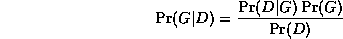

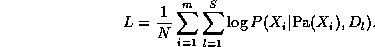
An exact Bayesian approach to model selection is usually unfeasible, since it involves computing the marginal likelihood P(D) = \sum_G P(D,G), which is a sum over an exponential number of models. However, we can use an asymptotic approximation to the posterior called BIC (Bayesian Information Criterion), which is defined as follows:

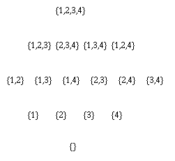
\sum_{k=0}^n \choice{n}{k} = 2^n
such sets, which can be
arranged in a lattice as shown below for n=4.
The problem is to find the highest scoring point in this lattice.
There are three obvious ways to search this graph: bottom up, top down, or middle out. In the bottom up approach, we start at the bottom of the lattice, and evaluate the score at all points in each successive level. We must decide whether the gains in score produced by a larger parent set is ``worth it''. The standard approach in the reconstructibility analysis (RA) community uses the fact that \chi^2(X,Y) \approx I(X,Y) N \ln(4), where N is the number of samples and I(X,Y) is the mutual information (MI) between X and Y. Hence we can use a \chi^2 test to decide whether an increase in the MI score is statistically significant. (This also gives us some kind of confidence measure on the connections that we learn.) Alternatively, we can use a BIC score.
Of course, if we do not know if we have achieved the maximum possible score, we do not know when to stop searching, and hence we must evaluate all points in the lattice (although we can obviously use branch-and-bound). For large n, this is computationally infeasible, so a common approach is to only search up until level K (i.e., assume a bound on the maximum number of parents of each node), which takes O(n ^ K) time.
The obvious way to avoid the exponential cost (and the need for a bound, K) is to use heuristics to avoid examining all possible subsets. (In fact, we must use heuristics of some kind, since the problem of learning optimal structure is NP-hard \cite{Chickering95}.) One approach in the RA framework, called Extended Dependency Analysis (EDA) \cite{Conant88}, is as follows. Start by evaluating all subsets of size up to two, keep all the ones with significant (in the \chi^2 sense) MI with the target node, and take the union of the resulting set as the set of parents.
The disadvantage of this greedy technique is that it will fail to find a set of parents unless some subset of size two has significant MI with the target variable. However, a Monte Carlo simulation in \cite{Conant88} shows that most random relations have this property. In addition, highly interdependent sets of parents (which might fail the pairwise MI test) violate the causal independence assumption, which is necessary to justify the use of noisy-OR and similar CPDs.
An alternative technique, popular in the UAI community, is to start with an initial guess of the model structure (i.e., at a specific point in the lattice), and then perform local search, i.e., evaluate the score of neighboring points in the lattice, and move to the best such point, until we reach a local optimum. We can use multiple restarts to try to find the global optimum, and to learn an ensemble of models. Note that, in the partially observable case, we need to have an initial guess of the model structure in order to estimate the values of the hidden nodes, and hence the (expected) score of each model; starting with the fully disconnected model (i.e., at the bottom of the lattice) would be a bad idea, since it would lead to a poor estimate.
The standard approach is to keep adding hidden nodes one at a time, to some part of the network (see below), performing structure learning at each step, until the score drops. One problem is choosing the cardinality (number of possible values) for the hidden node, and its type of CPD. Another problem is choosing where to add the new hidden node. There is no point making it a child, since hidden children can always be marginalized away, so we need to find an existing node which needs a new parent, when the current set of possible parents is not adequate.
\cite{Ramachandran98} use the following heuristic for finding nodes which need new parents: they consider a noisy-OR node which is nearly always on, even if its non-leak parents are off, as an indicator that there is a missing parent. Generalizing this technique beyond noisy-ORs is an interesting open problem. One approach might be to examine H(X|Pa(X)): if this is very high, it means the current set of parents are inadequate to ``explain'' the residual entropy; if Pa(X) is the best (in the BIC or \chi^2 sense) set of parents we have been able to find in the current model, it suggests we need to create a new node and add it to Pa(X).
A simple heuristic for inventing hidden nodes in the case of DBNs is to check if the Markov property is being violated for any particular node. If so, it suggests that we need connections to slices further back in time. Equivalently, we can add new lag variables and connect to them.
Of course, interpreting the ``meaning'' of hidden nodes is always tricky, especially since they are often unidentifiable, e.g., we can often switch the interpretation of the true and false states (assuming for simplicity that the hidden node is binary) provided we also permute the parameters appropriately. (Symmetries such as this are one cause of the multiple maxima in the likelihood surface.)
Classical control theory is mostly concerned with the special case where the graphical model is a Linear Dynamical System and the utility function is negative quadratic loss, e.g., consider a missile tracking an airplane: its goal is to minimize the squared distance between itself and the target. When the utility function and/or the system model becomes more complicated, traditional methods break down, and one has to use reinforcement learning to find the optimal policy (mapping from states to actions).
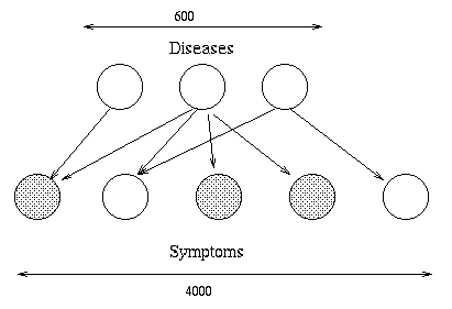
BNs originally arose out of an attempt to add probabilities to expert systems, and this is still the most common use for BNs. A famous example is QMR-DT, a decision-theoretic reformulation of the Quick Medical Reference (QMR) model.
Another interesting fielded application is the Vista system, developed by Eric Horvitz. The Vista system is a decision-theoretic system that has been used at NASA Mission Control Center in Houston for several years. The system uses Bayesian networks to interpret live telemetry and provides advice on the likelihood of alternative failures of the space shuttle's propulsion systems. It also considers time criticality and recommends actions of the highest expected utility. The Vista system also employs decision-theoretic methods for controlling the display of information to dynamically identify the most important information to highlight. Horvitz has gone on to attempt to apply similar technology to Microsoft products, e.g., the Lumiere project.
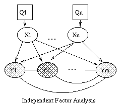
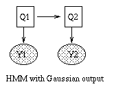
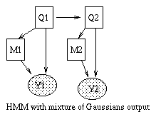
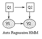
Special cases of BNs were independently invented by many different communities, for use in e.g., genetics (linkage analysis), speech recognition (HMMs), tracking (Kalman fitering), data compression (turbocodes), etc.
For examples of other applications, see the special issue on UAI of Proc. ACM 38(3), 1995.