
Assignment 1: Image Filtering and Hybrid Images
Due: At the end of the day 11:59pm, Monday, January 30th, 2023.
The purpose of this assignment is to get some initial experience with Python and to learn the basics of constructing and using linear filters.
There are different ways to import libraries/modules into Python. Styles and practices vary. For consistency (and to make life easier for the markers) you are required to import modules for this assignment exactly as follows:
        from PIL import Image
        import numpy as np
        import math
        from scipy import signal
        import cv2
If you are using Jupyter Notebook with Google Colab or on your personal machine, you will, in addition, would also want to import:
from IPython.display import Image
HINT: Review Assignment 0 for the basics of reading/writing images, converting colour to greyscale, and converting PIL images to/from Numpy arrays. Recall that visualizing imagies in regular Python and in Jupyter differs a bit. In regular Python you can use img.show() and in Jupyter you can use display(img).
Hand in all parts of this assignment using Canvas (both the code and PDF file as specified). To get full marks, your functions (i.e., *.py or *.ipynb files) must not only work correctly, but also must be clearly documented with sufficient comments for others to easily use and understand the code. You will lose marks for insufficient or unclear comments. In this assignment, you also need to hand in scripts showing tests of your functions on all the cases specified as well as the images and other answers requested. The scripts and results (as screenshots or otherwise) should be pasted into a single PDF file and clearly labeled. If you are using Jupyter, assuming you set things up correctly, you should be able to simply pint the notebook into a PDF file for submission. Note that lack of submission of either the code or the PDF will also result in loss of points.
The assignment
Part 1: Written Questions(6 points)
In this part of the assignment, you will be practicing filtering by hand on a given "image". You may find the questions here (if you are familiar with LaTex, feel free to use the following template to generate the answers). Annotate your results on the PDF. During submission, you will merge this PDF with your report. Make sure that you put this right after your report cover page.
Part 2: Gaussian Filtering(35 points)
-
(3 points)In CPSC 425, we follow the convention that 2D filters always have an odd number of rows and columns (so that the center row/column of the filter is well-defined).
As a simple warm-up exercise, write a Python function, ‘boxfilter(n)’, that returns a box filter of size n by n. You should check that n is odd, checking and signaling an error with an ‘assert’ statement. The filter should be a Numpy array. For example, your function should work as follows:
        >>> boxfilter(5)
        array([[ 0.04,  0.04,  0.04,  0.04,  0.04],
               [ 0.04,  0.04,  0.04,  0.04,  0.04],
               [ 0.04,  0.04,  0.04,  0.04,  0.04],
               [ 0.04,  0.04,  0.04,  0.04,  0.04],
               [ 0.04,  0.04,  0.04,  0.04,  0.04]])

        >>> boxfilter(4)
        Traceback (most recent call last):
          ...
        AssertionError: Dimension must be odd
HINT: The generation of the filter can be done as a simple one-line expression. Of course, checking that n is odd requires a bit more work.
Show the results of your boxfilter(n) function for the cases n=3, n=4, and n=5.
-
(5 points)Write a Python function, ‘gauss1d(sigma)’, that returns a 1D Gaussian filter for a given value of sigma. The filter should be a 1D array with length 6 times sigma rounded up to the next odd integer. Each value of the filter can be computed from the Gaussian function, exp(- x^2 / (2*sigma^2)), where x is the distance of an array value from the center. This formula for the Gaussian ignores the constant factor. Therefore, you should normalize the values in the filter so that they sum to 1.
HINTS: For efficiency and compactness, it is best to avoid ‘for’ loops in Python. One way to do this is to first generate a 1D array of values for x, and map this array through the density function. Suppose you want to generate a 1D filter from a zero-centered Gaussian with a sigma of 1.6. The filter length would be odd(1.6*6)=11. You then generate a 1D array of x values [-5 -4 -3 -2 -1 0 1 2 3 4 5] and pass the 1D array through the given density function exp(- x^2 / (2*sigma^2)).
Show the filter values produced for sigma values of 0.3, 0.5, 1, and 2.
-
(5 points)Create a Python function ‘gauss2d(sigma)’ that returns a 2D Gaussian filter for a given value of sigma. The filter should be a 2D array. Remember that a 2D Gaussian can be formed by convolution of a 1D Gaussian with its transpose. You can use the function ‘convolve2d’ in the Scipy Signal Processing toolbox to do the convolution. You will need to provide signal.convolve2d with a 2D array. To convert a 1D array, f, to a 2D array f, of the same size you use ‘f = f[np.newaxis]’
Show the 2D Gaussian filter for sigma values of 0.5 and 1.
-
(10 points)(a) Write a function ‘convolve2d_manual(array, filter)’ that takes in an image (stored in `array`) and a filter, and performs convolution to the image with zero paddings (thus, the image sizes of input and output are the same). Both input variables are in type `np.float32`. Note that for this implementation you should use two for-loops to iterate through each neighbourhood.
(b) Write a function ‘gaussconvolve2d_manual(array,sigma)’ that applies Gaussian convolution to a 2D array for the given value of sigma. The result should be a 2D array. Do this by first generating a filter with your ‘gauss2d’, and then applying it to the array with ‘convolve2d_manual(array, filter)’
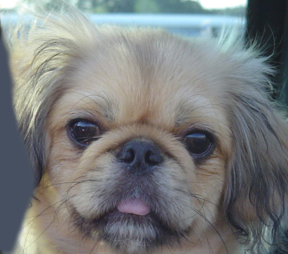
(c) Apply your ‘gaussconvolve2d_manual’ with a sigma of 3 on the image of the dog. Download the image (right-click on an image in your browser and choose “save as”). Load this image into Python, convert it to a greyscale, Numpy array and run your ‘gaussconvolve2d’ (with a sigma of 3). Note, as mentioned in class, for any image filtering or processing operations converting image to a double array format will make your life a lot easier and avoid various artifacts. Once all processing operations are done, you will need to covert the array back to unsigned integer format for storage and display.
(d) Use PIL to show both the original and filtered images.
-
(7 points)(a) Write a function ‘gaussconvolve2d_scipy(array,sigma)’ that applies Gaussian convolution to a 2D array for the given value of sigma. The result should be a 2D array. Do this by first generating a filter with your ‘gauss2d’, and then applying it to the array with signal.convolve2d(array,filter,'same'). The ‘same’ option makes the result the same size as the image.
The Scipy Signal Processing toolbox also has a function ‘signal.correlate2d’. Applying the filter ‘gauss2d’ to the array with signal.correlate2d(array,filter,'same') produces the same result as with signal.convolve2d(array,filter,'same'). Why does Scipy have separate functions ‘signal.convolve2d’ and ‘signal.correlate2d’? HINT: Think of a situation in which ‘signal.convolve2d’ and ‘signal.correlate2d’ (with identical arguments) produce different results.
(b) Apply your ‘gaussconvolve2d_scipy’ with a sigma of 3 on the image of the dog again. Follow instructions in part 4c for saving and loading the image.
(c) Use PIL to show both the original and filtered images.
-
(2 points)Experiment on how much time it takes to convolve the dog image above using your convolution implementation ‘gaussconvolve2d_manual’ and the scipy implementation ‘gaussconvolve2d’. Compare and comment on the performance using a sigma of 10.0. HINT: The following code shows you how to time a function. Also, depending on efficency of your implementation you may see different runtimes here compared to the the scipy implementation, that's OK. The key is thinking and explaining why you get a certain result.
import time t1 = time.time() # start timestamp operations() # some operations to time duration = time.time() - t1 # duration in seconds -
(3 points)Convolution with a 2D Gaussian filter is not the most efficient way to perform Gaussian convolution on an image. In a few sentences, explain how this could be implemented more efficiently taking advantage of separability and why, indeed, this would be faster. NOTE: It is not necessary to implement this. Just the explanation is required. Your answer will be graded for clarity.
Part 3: Hybrid Images(10 points)
(credit: this part of assignment is moddeled after James Hays course at GaTech)
Gaussian filtering produces a low-pass (blurred) filtered version of an image. Consequently, the difference between the original and the blurredlow-pass filtered counterpart results in a high-pass filtered version of the image. As defined in the original ACM Siggraph 2006 paper a hybrid image is the sum of a low-pass filtered version of the one image and a high-pass filtered version of a second image. There is a free parameter, which can be tuned for each image pair, which controls how much high frequency to remove from the first image and how much low frequency to leave in the second image. This is called the``cutoff-frequency''. In the paper it is suggested to use two cutoff frequencies (one tuned for each image) and you are free to try that, as well. In the starter code, the cutoff frequency is controlled by changing the standard deviation of the Gausian filter used in constructing the hybrid images.
We provide you with pairs of aligned images which can be merged reasonably well into hybrid images. The alignment is important because it affects the perceptual grouping (read the paper for details). We encourage you to create additional examples (e.g. change of expression, morph between different objects, change over time, etc.). See the hybrid images project page for some inspiration.
-
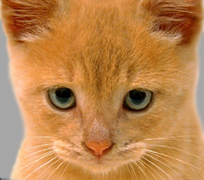
(3 points)Choose an appropriate sigma and create a blurred version of the one of the paired images. For this to work you will need to choose a relatively large sigma and filter each of the three color channels (RGB) separately, then compose the channels back to the color image to display. Note, you should use the same sigma for all color channels.

Original image Gaussian filtered low frequencies image -
(3 points)Choose an appropriate sigma (it is suggested to use the same as above) and create a high frequency version of the second from the two the paired images. Again you will operate on each of the color channels separately and use same sigma for all channels. High frequency filtered image is obtained by first computing a low frequency Gaussian filtered image and then subtracting it from the original. The high frequency image is actually zero-mean with negative values so it is visualized by adding 128 (if you re-scaled the original image to the range between 0 and 1, then add 0.5 for visualization). In the resulting visualization illustrated below, bright values are positive and dark values are negative.
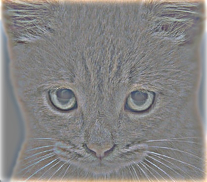
Original image High frequencies image -
(4 points)Now simply add the low and high frquency images (per channel). Note, the high frequency image that you add,should be the originally computed high friequency image (without adding 128; this addition is only done for visualizationes in the part above) You may get something like the following as a result:
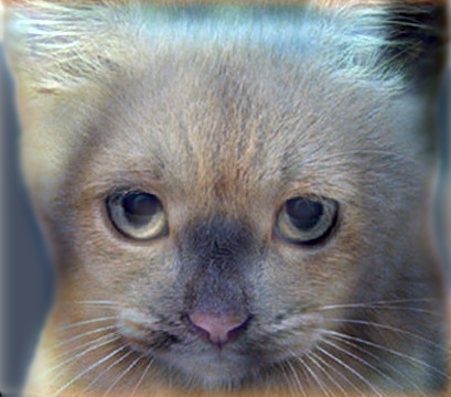
Depending on the sigma value your image may look different. Experiment with at least 3 provided sets of images or create your own hybrid. Illustrate results for 3 different values of sigma for each of the images.
Note: You may see speckle artifacts (individual pixels of bright color that do not match the image content) in the final hybrid image produced. You should be able to get rid of most, if not all, of them by clamping the values of pixels on the high and low end to ensure they are in the valid range (between 0 and 255) for the final image. You will need to do this per color channel. However, depending on the chosen value of sigma and specific set of images a few artifacts may remain. If you are unable to completely get rid of those artifacts that's OK. You will not be penalized for them, assuming all other parts of the assignment are done correctly and you made a reasonable attempt at producing a good result image (e.g., by implementing the clamping procedure described).
Part 4: Playing with Different Denoising Filters (9 points)
In this question, you are given two images affected by Gaussian noise and speckle noise box_gauss.png and box_speckle.png. You will apply Gaussian filter, bilateral filter, and median filter respectively to denoise the images. Use the existing implementation in the OpenCV library ‘cv2’. Specifically, you will use the functions ‘cv2.GaussianBlur’, ‘cv2.bilateralFilter’, and ‘cv2.medianBlur’. Please consult the OpenCV documentation for more details.
-
(6 points)Play with different combinations of parameters for each filter and show your best results for denoising. Include the best combinations of parameters for each filter and the corresponding resultant images in your report. Note that since you have two images and three filters, you will include a total of six denoised images.
-
(3 points)Now try to use the following combinations for the two images, and comment the pros and cons of using Gaussian, Bilateral, and Median filter. HINT: You might need to zoom in to see the artifacts clearly.
        import cv2
        cv2.GaussianBlur(img, ksize=(7, 7), sigmaX=50)
        cv2.bilateralFilter(img, 7, sigmaColor=150, sigmaSpace=150)
        cv2.medianBlur(img,7)
Deliverables
You will hand in your assignment ellectronically through Canvas. You should hand in two files, a file containig your code (i.e., *.py or *.ipynb file). This file must have sufficient comments for others to easily use and understand the code. In addition, hand in a PDF document showing scripts (i.e., records of your interactions with the Python shell) showing the specified tests of your functions as well as the images and other answers requested. The PDF file has to be organized and easily readible / accessible.
Assignments are to be handed in before 11:59pm on their due date.