Homework # 1

Learning Goal

Refresh your understanding of Bayesian inference. Work through a few manual review exercises that also communicate the inspiration behind the development of probabilistic programming languages and systems. Develop some familiarity with existing probabilistic programming languages and the relative ease of posing and solving Bayesian inference problems relative to the manual approach. This homework is long but will be “easy” intellectually if you have the appropriate level of probabilistic reasoning fluency and practical coding ability required to complete the course efficiently. Many have succeeded even when they found this first homework intellectually difficult or time-consuming from a coding perspective, however, be warned that the level of understanding required to really get what is going on rises very quickly, and the intellectual complexity of the coding tasks does as well.

Format

Please write up your answers using LaTeX and generate a .pdf. Include in this submitted report clickable \url{} links to and Weights and Biases (“wandb”) reports for the questions that demand it (3, 5, and 6). Please submit your homework to gradescope using the course code and instructions distributed in class. The homework is due at midnight PST on the evening of the indicated due date.

Questions

1) (2 points) Show that the Gamma distribution is conjugate to the Poisson distribution.

2) (2 points) Show that the Gibbs transition operator satisfies the detailed balance equation and as such can be interpreted as an MH transition operator that always accepts.

3) (10 points) Write code to compute the probability three ways that it is cloudy given that we observe that the grass is wet using this Bayes net model.

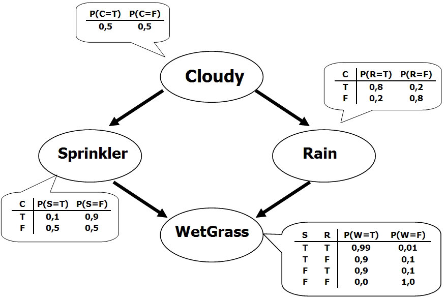
• By enumerating all possible world states and conditioning by counting which proportion are cloudy given the observed world characteristic, namely, that the grass is wet
• Using ancestral sampling and rejection
• Using Gibbs sampling

Start from the following Python support code

• Q3.py

Subsequent homework will assume familiarity and make extensive use of both PyTorch and Weights and Biases (“wandb”). Ensure that you sign up for Weights and Biases and are added to the cs532-2022 wandb team (send your wandb username or the email you used to sign up for wandb to the course wandb slack channel). For all subsequent homework, the hand-in results will take the form of wandb reports. Make such a report for the results of this homework question and put a clickable \url{} link to it in your LaTeX formatted hand-in.

4) (10 points) Consider the Bayesian linear regression model discussed in the lecture on graphical models

It has joint

$$p({\bf t},{\bf x},\sigma^2,{\bf w},\alpha) = \prod_{n=1}^N p(t_n | {\bf w}, x_n, \sigma^2)p({\bf w}|\alpha)$$

likelihood

$$t_n | {\bf w}, x_n, \sigma^2 \sim \mathrm{Normal}({\bf w}^T x_n,\sigma^2)$$

and prior

$${\bf w} | \alpha \sim \prod_{d=1}^D \mathrm{Normal}(0,\alpha) = \mathrm{Normal}({\bf w}|{\bf 0},\alpha{\bf I}_{d\times d})$$

Show and derive the updates required to

• perform MH within Gibbs on the blocks ${\bf w}$ and $\hat t$.
  • note that it is unnecessary to fall back on MH on either the ${\bf w}$ or $\hat t$ block. The reason exercise is being imposed on you is that when implementing generic inference algorithms later in the course (HW3 for instance) you will have to use a generic MH within Gibbs algorithm because analytic conditionals are, in fact, extremely uncommon. As a result truly understanding this question is critical for establishing the foundation for subsequent homeworks. While solving this problem you should think about how one might graphically determine the Markov blanket of a variable in an arbitrary graphical model.
• perform pure Gibbs on both ${\bf w}$ and $\hat t$.
  • relative to the preceding subquestion it now should be apparent that there are analytic forms for the conditionals of both blocks. What you should think about while doing this is whether or not it is common for such analytic conditionals to exist and why sampling efficiency is increased if they do exist.
• produce the analytic form of the posterior predictive.
  • here the thing to think about is that the return expression of probabilistic programs can be, for instance, a predicted quantity. This will be a posterior predictive quantity due to probabilistic programming semantics and you should, here, think about the Rao-Blackwellized integral that is be analytically computed here and why this is more efficient than, for instance, the sampling methods above

5) (10 points) Refer to HW3, Program 2. This program is written in the FOPPL syntax from the book and corresponds to a scalar version of question 4 of this homework. Starting from the Python scaffolding below, translate this FOPPL probabilistic program into Pyro and generate samples from the denoted joint posterior of slope and bias and the posterior predictive distribution of the model output (second “dimension” of data) given a new input value 0.0. Please write one or two sentences describing this model and applications and application settings in which such a posterior predictive distribution might be useful.

Start from the following Python support code

• Q5.ipynb

Note that this model is the same as the model in Q4 of this homework, in which we asked you to do manual inference algorithm design and derivation. Write a sentence or two in your response to this question about which approach to solving this problem is easier: Pyro or “by hand.” Write an additional sentence or two about potential disadvantages of the Pyro approach.

6) (OPTIONAL) (10 points; extra credit) Refer to HW2, Program 5, the “Bayesian neural network.” This program is written in the FOPPL syntax from the book. Starting from the Python scaffolding below, translate this FOPPL probabilistic program into STAN and generate samples from the denoted posterior of the network weights and the posterior predictive distribution of the network output given a new input value 6. Please write one or two sentences describing this model and reasons for why and applications in which such a posterior predictive distribution might be useful (hint: compare and contrast to simply fitting the neural network to the provided data and using the maximum likelihood model parameter estimate for prediction).

Start from the following Python support code

• Q6.ipynb