Motion compression by PCA combined with
high-degree polynomial regression
CPSC 533B course project
by Vadym Voznyuk
April 2003
1. Introduction
Motion data storage is an important issue in video games. There are various techniques that could be used to
compress motion data, but so far only the simplest, such as delta compression, have been employed by the game
development community.
Modern video game hardware does not allow anything much more powerful yet, but this should change in future.
In this project we present a simple framework for more advanced compression methods. Our work introduces a notion of
compression pipeline as a chain of data processing modules. By combining low-pass filtering, principal component analysis and
polynomial regression, we can achieve substantial data compression, although not without some drawbacks.
2. Motivation and theory
Delta compression of motion data, employed by the video games
today, is one of the most simple compression techniques. Its analogy is the
ADPCM compression of audio data. Core idea of delta compression is to store
differences (deltas)
between samples instead of samples themselves. In case of low-frequency motion
data, i.e. where motion curves are smooth, delta compression yields decent
results. However, it does not exploit correlation between character limbs
during motion.
This is where principal component analysis [3] comes handy. If we represent motion data as a matrix, we can do SVD (singular value
decomposition)
and obtain a set of singular values, whose magnitude indicates how important
is the particular component in the whole matrix. By cutting off less important
components, we can represent slightly altered version of original matrix
with less data.
Still, PCA itself is just one stage in the pipeline, although the main one. It is preceded by low-pass filtering or smoothing and
followed by polynomial regression.
Smoothing gets rid of the high-frequency components in motion, thus driving
less important principal components almost to zero. Polynomial regression
is something similar to spline interpolation [1] but not quite. Unlike cubic
splines, we are focused on piecewise polynomials of much higher degrees than
just cubics.
3. PCA and polynomial regression
The core of our framework is a combination of principal component
analysis (PCA) and polynomial regression [2]. PCA does preliminary stage
of dimensionality reduction, exploiting inherent correlation between character
limbs. The set of principal component
curves produced by PCA is then approximated by a set of piecewise polynomials of high degree.
3.1 Why PCA?
Since we use human motion capture data in our experiments, we will focus on motion of humans. Human character limbs
move more or less synchronously most of the time. Therefore, quite a few degrees of freedom in a human skeleton just follow
each other according to some locomotion pattern. We can exploit that and try to remove as much degrees of freedom as possible.
Let us suppose our motion data is represented as a rectangular matrix A. Singular value decomposition allows us to
factorize A into three special matrices: A=USV. U and V are our new principal component
matrices, and S is a diagonal matrix, with singular values on the diagonal. For a data matrix A representing human
motion clip, the graph of its singular values looks like this:

Figure 1. Graph of the singular value set (diagonal of S) for the typical human motion data matrix A.
Figure 1 demonstrates that human motion consists of one very large
component, about a dozen of significantly smaller ones and the rest is almost
zero. In other words, this graph tells us there is a lot of redundancy in
the matrix A and we can squeeze it significantly
without losing much of the motion detail.
How do we squeeze the matrix? The most straightforward way is to cut off
components starting from some reasonable number, for example, 20. If we cut
off components from 21-st till the last, we will get a set of principal components, which constitute the essence of our
motion data. We do this by replacing product of matrices S and V by one matrix D. Now our SVD equation is
A=UD. The only step left is to cut off columns of U starting from 21-st and also cut off rows of D also
starting with 21-st. The result of this operation is a set of two smaller matrices, Uc and Dc, product of which
gives us slightly altered matrix A.
As a demonstration of correlation removing ability of PCA we will include
two illustrations below. One shows the original 128 curves of the motion
clip, while the other is a graph of 10 principal components of that clip's
motion data matrix.
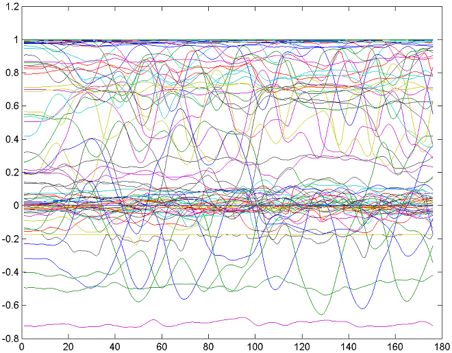
Figure 2. Graph of the original motion data matrix A. This is a clip of human run.
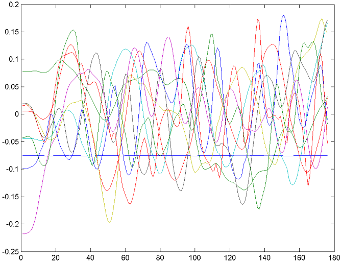
Figure 3. Graph of the 10 principal components of A.
Note that while figure 2 depicts many highly correlated curves
that show synchronous and interdependent motion of human limbs during run,
figure 3 has no correlated curves at all.
3.2 Why polynomial regression?
In the beginning we had original set of correlated curves stored in the matrix A. After PCA we have a set of uncorrelated
principal component curves stored in matrix Uc plus a transformation matrix Dc. The transformation matrix is a set
of orthogonal basis vectors, so we just leave it as is. Principal component curves in Uc, however, could be approximated by
some equations. We chose the approximation model to be polynomial, due to its simplicity and ability to approximate curves with
multiple extrema.
3.3 What about "high-degree"?
Common approaches to piecewise curve approximation employ quadratic
or cubic curves. This is also true for spline approximation or interpolation.
We depart from this practice and limit the polynomial degree by much higher
numbers (maximum 30 in current implementation). This gives us opportunity
to explore approximation of large curves with many extrema by a single polynomial.
In theory, such occasions could lead to higher compression ratio, since single
high degree polynomial will always have fewer coefficients than a set of
piecewise quadratics or cubics approximating the same curve.
4. Implementation
Our compression framework is implemented as two separate modules.
The first is the motion loader and player, the second is a set of Matlab scripts
performing actual data processing tasks. Motion player fftgraphd.exe
is a binary executable for Windows, it launches a local copy of Matlab when
started. Then it establishes COM link with Matlab and uploads motion data
into the Matlab's workspace as a rectangular matrix. The Matlab script mfit.m provides GUI for the data manipulation tasks. The GUI
window together with brief description of its controls is depicted below:
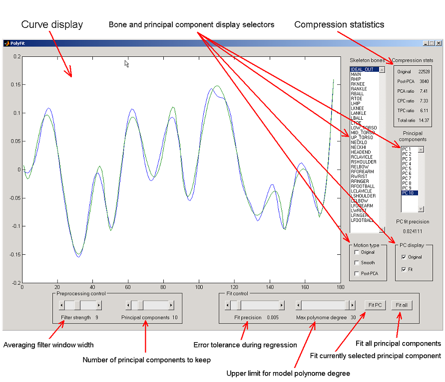
Figure 4. GUI window is a framework's front-end, here the user performs all the data manipulation.
Besides UI controls in the window above, there are also two important controls in the motion player. The player, when started,
will just display the character performing. To bring on the controls, the user has to press Enter on the keyboard.
After that the control menu appears in the upper left corner of the player window.
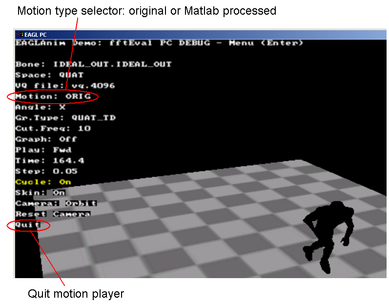
Figure 4. Section of the motion player window with the control menu. Two important controls are circled.
Note that the motion player cannot be closed by the standard Windows
close button in the upper right corner of the window. The user has to select
Quit item in the menu and press spacebar on the keyboard.
To switch between original and Matlab processed motion, the user has to select the Motion
menu item with up and down arrows, and use left/right arrows to switch motion
type. Left and middle mouse buttons allow the user to control the camera
- orbiting, panning and zooming.
To start the system user has to start the motion player first, by issuing command fftgraphd filename in the
operating system's command prompt, where filename points to the motion data file. After that two windows appear on the screen.
One is the player's window and the other is the Matlab COM server window. Now the user has to change to the directory with
mfit.m and issue command mfit in
the Matlab window. The GUI window comes up and the system is ready to process
motion data. To load another motion clip, quit the player, reload it with
a new motion data file and also restart GUI by closing it and typing mfit in Matlab again. After each data processing session you can observe the
resulted motion by switching to the motion player and choosing original motion and then Matlab processed one. This will refresh
motion data in the player by reloading it from Matlab.
The set of motion data files included with the system is described below.
255_3_or.o - run followed by sharp turn and fall
255_3_st.o - slightly crouched run followed by collision, roll and fall
256_1_or.o - plain run
256_1_st.o - run, collision, squat and run in the opposite direction
257_3_or.o - run, collision and fall
257_3_st.o - run followed by violent collision, short flight in the air and fall
258_3_or.o - run with mild collision in the middle
258_3_st.o - run, sharp turn with crouching and almost losing balance followed by run in the opposite direction
259_2_or.o - run and fall forward
259_2_st.o - run, collision, losing balance, fall and roll over
4.1 Curve and principal component visualization
The largest UI control in the GUI window is a curve drawing area. It displays both original motion curves as well as principal
component curves. Five checkboxes near the bottom right corner of GUI window control which curves are being displayed and which
stay hidden. Motion type group of checkboxes controls display of the original motion curves, smoothed curves and
post-PCA curves. Read on to understand what they are. PC display checkboxes control the appearance of the principal
component curves, both original and fit ones.
4.2 Compression pipeline
Motion data are compressed in the three-stage pipeline.
- Stage 1: smoothing. Done by the averaging low-pass filter. Gets rid
of high-frequency motion components, thus making it possible to keep less
principal components of the motion data matrix.
- Stage 2: dimensionality reduction through PCA. Done by singular value decomposition followed by pruning unimportant
components of the motion data matrix.
- Stage 3: high-degree polynomial regression. Done by linear least
squares polynomial fitting. Note that we try to fit the principal component
curves obtained in stage 2, not the original motion ones.
4.2.1 Curve smoothing
This is quite simple operation. Each original motion curve is
smoothed by the averaging filter. The filter window width determines how
smooth the resulting curves will be. This parameter is controlled by the
Filter strength slider at the bottom left
of the GUI window. The wider is the window - the smoother are the resulting curves.
4.2.2 Finding principal components
This is defining parameter of the whole system. It sets the principal components keeping threshold. All the less important
components above that threshold will be pruned. It is controlled by the Principal components slider to the
right of the Filter strength slider. The more principal components are being kept - the less is the compression
ratio and the better is the resulting motion quality.
4.2.3 Controlling polynomial regression parameters
There are two parameters that user can adjust. The first is error
tolerance (or precision) of the fit, and the second is the maximal polynomial
degree allowed during fit. Minimal value is 3 and maximum is 30. We found
that most of the time value around 22-24 produces reasonably good results.
Fit precision calculation code in the system is a bit tricky. It tries to adjust the fit error tolerance according to the
importance of the particular curve, or its weight in restoring matrix A.
Obviously, human skeleton joints have various importance in locomotion. For
example hip or waist joints are much more important during run or jump than
finger or neck joints. On the other hand, the same effect is observed after
PCA - certain singular values have much larger magnitude than the others.
Hence we have to do our best to avoid flat error tolerance where it is set to the same value for all curves being fit.
Adjustment of error tolerance according to the curve weight is done in two
passes. First, the tolerance is calculated depending on the span of the curve, i.e. difference between its maximal and minimal
values. Naturally, the curves corresponding to larger singular values will
have smaller span than curves corresponding to small singular values. Our
code takes that into account so that the most important curve corresponding
to the largest singular value is given the tightest possible error tolerance,
while the least important curve will be approximated quite loosely. Second
pass is done over the results of the first pass. Now we adjust error tolerance
for each curve once more, except for the most important one. This time we
employ singular values directly (instead of the curve span) as a guide in
the process. We multiply each error tolerance by the fixed fraction of the
reciprocal of singular value for that curve. Currently fraction coefficient
is set to 0.2, this value seemed to be optimum during experiments with mocap
data compression. The smaller is the singular value - the larger is its reciprocal
and hence the looser will be the polynomial approximation.
All these highly technical details mean one important thing - value of a slider Fit precision is just a guide.
The user suggests the system how precise he wants the fit to be, and the system distributes error tolerance values among curves
according to that guide and curve importance.
4.3 Compression statistics
Upper right corner of the GUI window feature a compression statistics pane. It has the following gauges:
- Original. Number of samples in the original motion data matrix A.
- Post-PCA. Number of samples in the pruned principal component matrix Uc.
- PCA ratio. Ratio between two values above. The larger it is - the better is PCA compression.
- CPC ratio. Current Principal Component ratio. Ratio between a number of polynomial coefficients
necessary to restore a currently selected principal component curve and a number of samples in that curve. The larger
value indicates better compression.
- TPC ratio. Total Principal Component ratio. This is the same as above but summarized over all the principal
component curves.
- Total ratio. Ratio between the total number of polynomial coefficients for all the principal component curves
plus the number of samples in the transformation matrix D and the number of samples in the original motion data
matrix A. In fact, this is reasonable approximation to the real compression ratio produced by the production-quality system
similar to our prototype. The larger is this value - the better is overall compression.
These indicators (except the first one) are updated every time PCA or polynomial fit have been performed.
5. Experiments with EA mocap data
We conducted extensive experiments with various motion clips taken
from the Electronic Arts mocap studio. We will include some results below.
The motion clips we analyze are the plain human run and the run followed
by sharp turn and fall.
5.1 Run, turn and fall
This clip turned out to be very tough for our framework to deal
with. It has two nasty features that do not allow us to achieve high compression
ratio. Each of those features works against one specific approach. One hurts
the ability of the system to do dimensionality reduction through PCA, while
the other turns high-degree polynomial regression into nightmare.
First, it has a lot of uncorrelated data in it, because run plus sharp turn
plus fall constitutes "chaotic" limb motion. Chaotic in the sense "uncorrelated".
This forces us to keep more principal components in matrix Uc.
Second, it has several seconds of time right at the end of the clip
where character just lies on the floor, without any motion. Both the original
motion curves and principal component curves turn into straight lines during
this. Approximating straight line by a high-degree polynomial is by definition
a meaningless waste of ammo. The picture below illustrates the point.
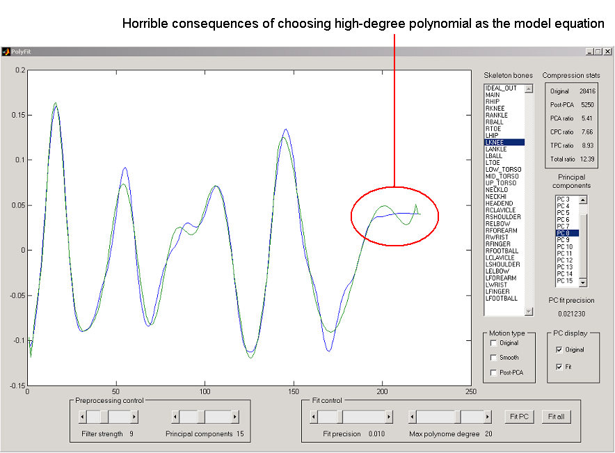
Figure 5. What happens when fitting polynomial meets straight line.
Due to these inconvenient clip features we had to increase both
the number of principal component (PC) curves and the error tolerance. After
we set the number of PC curves to 15 and error tolerance to 0.001, the compressed
motion started look reasonable. The compression ratio has suffered of course.
We couldn't achieve TPC ratio higher than 11 without making resulting motion
look very unnatural.
5.2 Plain run
This motion clip is on the opposite side of the scale. It does
not have either no-motion fragments or uncorrelated motion fragments. Because
of that we could lower PC curve number to 10 and also loosen error tolerance
compared to the previous example. Result - TPC ratio in the range of 14-14.5,
depending on how much "unnatural feel" we want in the result.
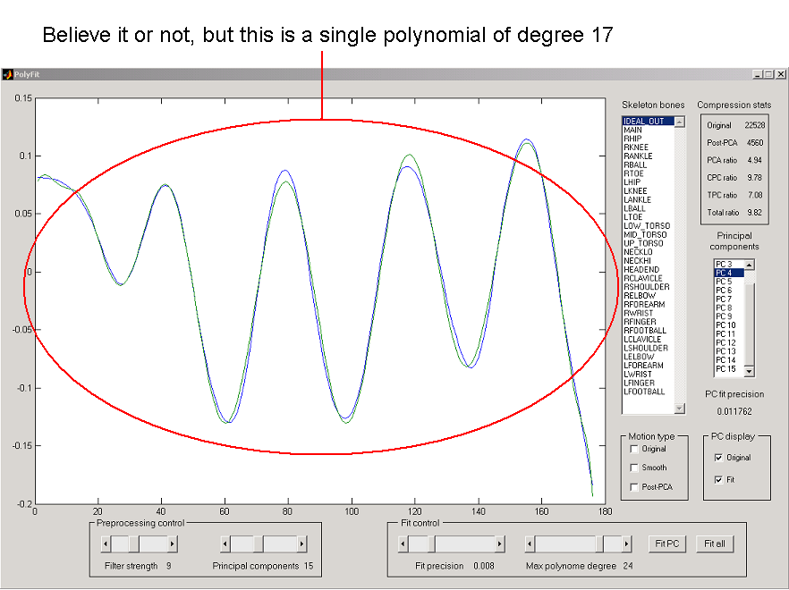
Figure 6. If only all the PC curves were always as nice as this one.
Figure 6 shows that fitting the whole curve with one high-degree
polynomial is not a fantasy. Unfortunately, it turned out that such nicely
"fittable" curves are rather rare. Most of them are approximated in a piecewise
fashion, which does not benefit TPC ratio.
6. Conclusion
We have built a motion compression framework prototype demonstrating
a combination of two simple motion compression techniques. Combining polynomial
regression with principal component analysis poses some challenges, some
of which are hard to overcome while the others are not. The problem of weighted
error tolerance could be solved without a lot of hard work, but the issue
of "wiggly" polynomials unable to approximate straight lines, seems to be
unsolvable in principle. A serious
disadvantage of our framework is total lack of scientific measure of motion
quality. All measurements were done just by observing compressed motion in
the player. The author admits that all that has been said about "reasonable"
motion quality is highly subjective matter. However, finding and proving
good metric for compressed motion quality would constitute a topic of research
by itself.
Another major disadvantage is the choice of model equations. Polynomials are not only the poor approximation equations for many
types of curves common in animation (such as much discussed above straight lines), they also could be extremely expensive as a
tool of compression for video games. Evaluating numerous polynomials of degrees between 8 and 18 for a small motion clip is not
the way to go.
The last important thing worth mentioning is recurring again and again importance of storing certain constraints together with
animation data. Foot-floor contact points are the best example. By storing and using them in compression, we could possibly
avoid main artifact occurring during compression - sliding feet. It is likely that we could compensate for additional storage
requirements for these constraints by applying more powerful and more lossy compression methods.
7. References
S. Sudarsky and D. House. Motion capture data manipulation and reuse via B-splines.
D. Cuthbert and F. S. Wood. Fitting equations to data. John Wiley & Sons, 1980.
Z. Ghahramani and G. E. Hinton. Parameter estimation for linear dynamical systems.