Dynamics of a Floating Object
Project report for CPSC 533B: Algorithmic Animation
Ken Deeter
 |
 |
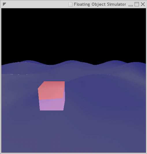
| Solid rendering |
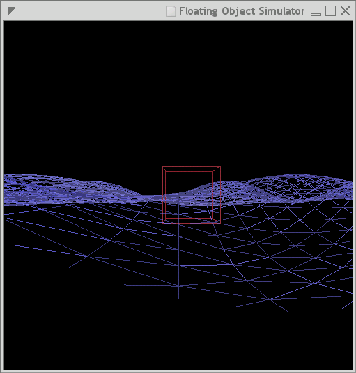
Wireframe rendering |
1. Introduction
The simple goal of this project was to build a dynamics simulator that
models the interaction of solid objects with water (or other
liquids). Although there has been much work in the areas of simulating
rigid body dynamics, as well as water, there has not been a
significant amount studying the interaction of the two. Only the most
complex of commercial particle system simulators provide support for
modeling the complicated interaction between solid objects, with
non-solid fluids.
2. Relevant Work
Much effort past has gone into modeling many different kinds of
liquids. Approaches range from computational fluid dynamics,
procedurally generated liquid surfaces, and approximations or
simplifications of the Navier-Stokes equation. Study of this topic
dates back to several reports such as [FOURNIER] and [PEACHY].
A recent paper by Foster and Fedikw [FOSTER], describe a system which can
handle moving solid objects, but does not model the forces that a
fluid exerts on that object.
As for the physics of floating objects, various levels of
understanding have been around since the time of Archimedes. The ideas
referenced in this project (in the domain of physics and mechanics)
can be found in any standard physics textbook or related web reference.
3. Approach and Implementation
In order to make the project feasible in the limited timeframe,
complexity of the model was reduced down to its basics as much as
possible. This simple design assumes a height-field representation of
a surface of a deep body of water, with directional sinewaves
simulating water waves (with controllable amplitude, frequency, and
direction). Only one type of object, a simple cube, is
modeled. Although the size of the cube can be controlled, no other
aspects of the shape can be modified. The implementation, however,
does not make simulation of other shapes impossible. The cube was
chosen because it simplifies many of the calculations required in modeling
its interaction with a liquid. Both vertical and lateral forces are
modeled, but rotation of the cube is not taken into account, resulting
in a cube that is always "upright."(see future work)
To model the motion of solid objects in water, three main forces must
be computed.
- Buoyancy Force: According to Archimedes' principle, the net vertical
force on a submerged object is equal to the weight of the water
displaced.
- Drag Force: As an object moves through a liquid, a force
proportional to the velocity of the object, viscosity of the fluid,
and cross-sectional area of the object, exists that resists the
motion.
- Gravity: As in most real-world simulations, the gravity exerts
a constant downward force proportional to an object's mass
Calculating the Buoyancy Force
A true complete calculation of a buoyancy force on an object involves
integrating the pressure exerted by the surrounding water over the
object's surface. Because static pressure at a point in water depends
on depth, a net upward force results from the fact that the surfaces
on the shallower end of an object experience less pressure than the
deeper surfaces.
For completely submerged objects, this net force is roughly equal to
the weight of the fluid displaced by the object, or in other words,
the volume of the object times the fluid's density.
For partially submerged objects, a slight approximation is necessary
to avoid calculating the surface integral. In my implementation, I
treat the partial submersion case in exactly the same manner as the
fully submerged case, except that the "weight of the fluid displaced"
is only calculated for the partial volume of the object that is
actually below the water's surface.
To account for the fact that the partially submerged portion of the
object may not necessariy correspond to the "lower" portion
of the object (which would imply that the resulting buoyancy force
would always be pointing "up"), the force is applied in a
direction obtained from the water surface's normal vector. This simple
approximation allows for somewhat realistic lateral movement of an
object at the water's surface, as if it is being pushed around by a
wave.
Calculating the Submerged Volume of the Cube
The most general method of calculating the volume of water displaced
by an object, is to divide its volume into many smaller sub-volumes,
and determe the depth of a point representing each sub-volume. If the
"height" coordinate (in world-space) of that point is lower
than the height of the water's surface at that point, then we can make
an approximation and treat the entire sub-volume as being
submerged. Summing up all such submerged sub-volumes will yield an
approximation of the total partial submerged volume.
In my implementation, I use a simpler method to approximate the
submerged volume of the cube. Because the cube is always upright, the
amount of submersion can be approximated by evaluating the height of
the water surface at each of vertically oriented edges of the cube.
Specifically, the approximation is computed as follows:
- Compute the depth of each of the four lower corners of the cube
- If a corner is found to be above the water of the surface, then
assign its corresponding vertical edge a submerged height value of
0. If it's depth is greater than the length of one of the edges of the
cube, then assign it a height value equal to the single edge length. Otherwise,
assign the edge a height value equal to the depth of the corner.
- Average the four height values, and multiply the average by
the area of the cube's base.
This approximation only works for relatively small cubes and
relatively low frequency water surfaces. In effect, it samples four
surface locations (for corners of a square), and approximates the
surface height across the square patch to be the average of the
heights at each of the four locations.
Calculating the Drag Force
The drag force on an object moving through a liquid is proportional to
the product of the square of its velocity, the density of the fluid,
and the cross-sectional area of the object. A constant is also
introduced, which depends on the shape of the object.
In this implementation, the three values mentioned above are
incorporated into the calculation of the drag force. The density of
water is fixed at 1000 kilograms per cubic meter and the cube's
cross-sectional area is approximated by the area of one of the cube's
faces.
Object-water collision
When an object collides into a water surface, a great portion of its
kinetic energy is transferred to the water, resulting in splashing and
waves. To simulate this loss of energy, a hard-coded percentage of the
cube's velocity is deducted when a collision with the water's surface
is detected. The percentage of determined empirically. A value of
approximately 90% appears to produce reasonable results.
Modeling Waves
Originally, I intended to use a method based on [HINSINGER] to model
the water waves. Although this model produced more realistic results,
it has one major problem: it is difficult, given an (x,y) coordinate
in the surface plane of the water, to determine the height of the
water at exactly that point. This is due to the fact that Hinsinger et
al.'s method distorts the (x,y) location of a point on the surface to
model the realistic elliptical motion actual water molecules.
In calculating buoyancy forces, it is necessary to often query the
height field for a water surface height value at an arbitrary position
(x,y) in the plane. Because of this requirement, I chose instead, to
use simple sinusoidal functions to model each wave, as they only
modify the height of each position on the surface, and not the lateral
position.
The tradeoff in realism is not show-stopping, especially for small
waves, and the added simplicity makes the computation much more
efficient. One idea that was retained from the implementation, is that
the water surface's normal vectors are always computed analytically,
providing for better results in both rendering and dynamics
computation.
Integration
The midpoint method (Heun's method) is used to acheive numerical
stability. The default maximum time increment for the integration is
100 milliseconds.
4. Results
Click here (2.2MB) to view a 15fps 24
second recording of the system in action. Note that, the actualy
system runs at full framerate (30fps+) on a pentium4 1.8ghz. The lower
framerate was required since framebuffer recording happens in
realtime. (NOTE: this file was encoded using the Divx4 codec)
The cube object modeled in this video has a mass of 200 kg, has 1 meter
length on each edge. As the equivalent weight of water for such a
volume is 1000kg, the object is fairly buoyant, and can be seen being
tossed into the air by passing waves.
In a second file (1.0MB), the same
object is shown being affected by a very large slow moving wave. (The slight
change in framerate is due to a rendering glitch)
5. Future Work
The work presented in this report can be extended in many
straightforward ways:
- Support for a variety of shapes. One need only solve the
submerged partial volume computation problem for each new shape.
- Support for multiple solid objects and interactions among them.
- Support for modeling rotation, torque, and angular velocity. A method similar to the
previously described integration method can be used to compute a net torque on the floating
object.
- Model effects of object on water. As of now, the system only models the
forces and effects of the water on the solid object. To be complete, the system
also needs to acount for perturbations to the water's surface caused
by the object's presence, including ripples and splashes.
- Better simulation of water. Although a more realistic simulation of water waves
was originally intended, a simpler method was chosen for
computational simplicity. In theory, however, any model of a body of water's surface can be
used for this type of simulation.
References
kdeeter cs ubc ca
Last modified: Fri Apr 25 03:03:59 PDT 2003