Each row represents a question, and each column represents one of the four students, in the order Cathy (1), Heather (2), Mark (3), and Allison (4). The color blue means the answer was correct, and red means the answer was wrong.
We will assume that the chance of a student answering a question
right is independent of the question (there are no 'hard' or
'easy' questions, and Allison/Heather don't make the same mistakes because they
studied together).
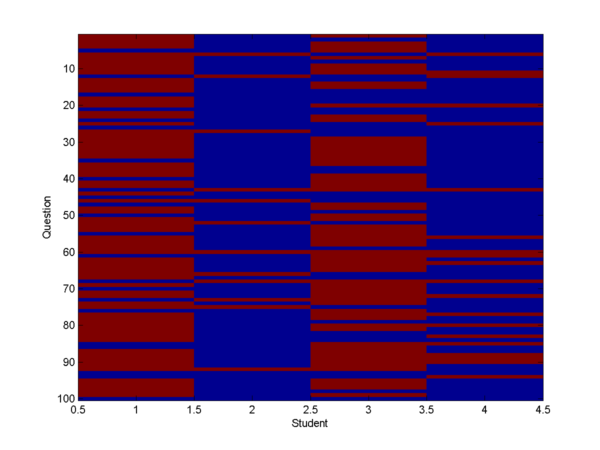
If we simulate 100 independent questions under this scenario, the results would
look something like:
Each row represents a question, and each column represents one of
the four students, in the order Cathy (1), Heather (2), Mark (3), and Allison
(4).
The color blue means the answer was correct, and red means the answer was wrong.
On the second test, the four students are placed in the same room. They are seated in the order Cathy-Heather-Mark-Allison, and can see the answers on the test next to them. Cathy (1) and Mark (3) assume that Heather (2) and Allison (4) studied for the exam (which they did), and Heather and Allison assume that Cathy and Mark also studied (even though they didn't), so everybody thinks that the person next to them will probably get the right answer. Below is the graph we will use to model this situation:

Since the students can see their neighbours' answers, and they think that their neighbours' answers carry information about the answers to the questions, the student's answers become dependent. Indeed, all of the students answers are dependent; even though Mark and Cathy do not sit next to each other, their answers are dependent because they both sit next to Heather. Even Cathy and Allison's answers are dependent, because a path exists between them in the graph. In UGMs, we say that two variables are independent if no path exists between them in the graph. In this case (and in many real-life applications), no variables are independent.
However, even though none of the four variables are independent, there are conditional independencies. For example, if we know the value of Heather's answer, then Mark and Cathy will be independent given this information. In UGMs, we say that two variables are conditionally independent if removing the conditioning variables from the graph makes the variables independent. In this case, if we remove the Heather node then there is no longer a path between Mark and Cathy in the graph.
In pairwise UGMs, the joint probability of a particular assignment to all the variables xi is represented as a normalized product of a set of non-negative 'potential' functions:
There is one potential function ('phi') for each node 'i', and each edge 'e'.
Each edge connects two nodes, 'ej' and 'ek'. In our example, the nodes are the individual students ('Cathy', 'Heather', 'Mark', 'Allison'), and we place edges between the students that sit next to each other ('Cathy-Heather', 'Heather-Mark', 'Mark-Allison'). Note that we only place edges between nodes that have a direct interaction, and we do not place edges between variables that only interact through an intermediate variable.
The 'node potential' function phii gives a non-negative weight to each possible value of the random variable xi. For example, we might set phi1('wrong') to .75 and phi1('right') to .25, which means means that node '1' has a higher potential of being in state 'wrong' than state 'right'. Similarly, the 'edge potential' function phie gives a non-negative weight to all the combinations that xej and xek can take. For example, in the above scenario students that sit next to each are more likely to have the same answer so we will give higher potentials to configurations where xej and xek are the same.
The normalization constant 'Z' is simply the scalar value that forces the distribution to sum to one, over all possible joint configurations of the variables:
This normalizing constant ensures that the model defines a valid probability distribution.
Given the graph structure and the potentials, UGM includes functions for three tasks:
nNodes = 4;
nStates = 2;
adj = zeros(nNodes,nNodes);
adj(1,2) = 1;
adj(2,1) = 1;
adj(2,3) = 1;
adj(3,2) = 1;
adj(3,4) = 1;
adj(4,3) = 1;
edgeStruct = UGM_makeEdgeStruct(adj,nStates);
The edgeStruct is designed to efficiently support three types of queries:
edgeStruct.nStates

ans =

     2
     2
     2
     2
In this case, all four nodes have 2 possible states that they can be in.
The edgeStruct.edgeEnds matrix is a nEdges-by-2 matrix, where each row of the matrix gives the two nodes associated with an edge. In our case, displaying this nEdges-by-2 matrix gives:
edgeStruct.edgeEnds

ans =

     1     2
     2     3
     3     4
As a specific example of how this is used, we can find the nodes associated with edge '2' as follows:
edge = 2;
edgeStruct.edgeEnds(edge,:)

ans =

     2     3
This means that edge '2' is an edge between nodes '2' and '3' (i.e. this is the 'Heather-Mark' edge).
The function UGM_getEdges uses the edgeStruct.V and edgeStruct.E vectors of pointers to allow us to quickly perform the reverse operation. In particular, the following command lets us find all edge numbers associated with a node 'n':
n = 3;
edges = UGM_getEdges(n,edgeStruct)

edges =

     2
     3
In this case we set 'n' to '3' (corresponding to 'Mark'), and the query reveals that node '3' is associated with edge '2' (this is the edge between '2' and '3', the 'Heather-Mark' edge) and '3' (this is the edge between '3' and '4', the 'Mark-Allison' edge). We can subsequently find the neighbours of node '3' in the graph by looking up rows '2' and '3' in the edgeStruct.edgeEnds matrix. For example, we can get the list of neighbours of node 3 using:
nodes = edgeStruct.edgeEnds(edges,:);
nodes(nodes ~= n)

ans =

     2
     4
This means that node '3' ('Mark') is neighbors with nodes '2' ('Heather') and '4' ('Allison').
To make the node potentials, we first consider writing the chance of getting an
individual question right in the first test as a table:
| Student | Right | Wrong |
| Cathy | .25 | .75 |
| Heather | .9 | .1 |
| Mark | .25 | .75 |
| Allison | .9 | .1 |
nodePot = [.25 .75
    .9 .1
    .25 .75
    .9 .1];
However, note that because of the way UGMs are normalized, we can multiply any row of the nodePot matrix by a positive constant without changing the distribution. Since we will be verifying things by hand below, we'll multiply the rows by some convenient constants so that we get some nice whole numbers. This gives us the following nodePot:
nodePot = [1 3
    9 1
    1 3
    9 1];
Keep in mind that these these two node potentials are equivalent, in the sense that they will lead to the same distribution.
| n1\n2 | Right | Wrong |
| Right | 2/6 | 1/6 |
| Wrong | 1/6 | 2/6 |
maxState = max(edgeStruct.nStates);
edgePot = zeros(maxState,maxState,edgeStruct.nEdges);
for e = 1:edgeStruct.nEdges
   edgePot(:,:,e) = [2 1 ; 1 2];
end
Although we have assumed that the two-by-two edge potentials are the same for all three edges and that they are symmetric, UGM also works for models where this is not the case. However, as with node potentials note that potentials can not be negative.
To illustrate these tasks, it will be helpful if we expand the distribution represented by the UGM into a big table that contains all configurations of right/wrong for each student. In the table below, np(i) is short for the node potential of the answer of student 'i', and ep('e') is short for the edge potential of edge 'e':
| Cathy | Heather | Mark | Allison | np(1) | np(2) | np(3) | np(4) | ep(1) | ep(2) | ep(3) | prodPot | Probability | |||
| right | right | right | right | 1 | 9 | 1 | 9 | 2 | 2 | 2 | 648 | 0.17 | |||
| wrong | right | right | right | 3 | 9 | 1 | 9 | 1 | 2 | 2 | 972 | 0.26 | |||
| right | wrong | right | right | 1 | 1 | 1 | 9 | 1 | 1 | 2 | 18 | 0.00 | |||
| wrong | wrong | right | right | 3 | 1 | 1 | 9 | 2 | 1 | 2 | 108 | 0.03 | |||
| right | right | wrong | right | 1 | 9 | 3 | 9 | 2 | 1 | 1 | 486 | 0.13 | |||
| wrong | right | wrong | right | 3 | 9 | 3 | 9 | 1 | 1 | 1 | 729 | 0.19 | |||
| right | wrong | wrong | right | 1 | 1 | 3 | 9 | 1 | 2 | 1 | 54 | 0.01 | |||
| wrong | wrong | wrong | right | 3 | 1 | 3 | 9 | 2 | 2 | 1 | 324 | 0.09 | |||
| right | right | right | wrong | 1 | 9 | 1 | 1 | 2 | 2 | 1 | 36 | 0.01 | |||
| wrong | right | right | wrong | 3 | 9 | 1 | 1 | 1 | 2 | 1 | 54 | 0.01 | |||
| right | wrong | right | wrong | 1 | 1 | 1 | 1 | 1 | 1 | 1 | 1 | 0.00 | |||
| wrong | wrong | right | wrong | 3 | 1 | 1 | 1 | 2 | 1 | 1 | 6 | 0.00 | |||
| right | right | wrong | wrong | 1 | 9 | 3 | 1 | 2 | 1 | 2 | 108 | 0.03 | |||
| wrong | right | wrong | wrong | 3 | 9 | 3 | 1 | 1 | 1 | 2 | 162 | 0.04 | |||
| right | wrong | wrong | wrong | 1 | 1 | 3 | 1 | 1 | 2 | 2 | 12 | 0.00 | |||
| wrong | wrong | wrong | wrong | 3 | 1 | 3 | 1 | 2 | 2 | 2 | 72 | 0.02 |
This corresponds to finding the row in the 'prodPot' column that has the largest value. In this case, the largest value is 972, for the configuration (Cathy:wrong, Heather: right, Mark: right, Allison: right). This configuration happens approximately 26% of the time. In contrast, the most likely scenario under test 1 where the students were independent was (Cathy: wrong, Heather: right, Mark: wrong, Allison: right), which happens around 19% of the time in test 2.
For small graphs (where it is feasible to enumerate all possible states), we can find the optimal decoding in UGM using:
optimalDecoding = UGM_Decode_Exact(nodePot,edgePot,edgeStruct)

optimalDecoding =

     2
     1
     1
     1
For example, one inference task would be to calculate how often Mark gets the question right. In test 1, this was trivially 25% of the time. In test 2, we do this by adding up the 'prodPot' for each configuration where Mark got the question right, then dividing by Z. In this case, adding up the potentials for each configuration gives 648+972+18+108+36+54+1+6=1843, and dividing this by 3790 gives approximately 0.49. Thus, Mark is almost twice as likely to get the right answer in test 2 than test 1. Cathy also benefits from sitting by Heather, her marginal increases to 0.36. She doesn't get as big of a benefit in test 2 because she only has one neighbour. Allison's marginal probability of being right in test 2 is 0.88, down from 0.9 in test 1 (because of Mark's bad answers). Heather is affected even more by being beside two bad neighbours, her marginal probability of being right is 0.84.
Note the difference between decoding and inference. In the most likely configuration, Mark gets the right answer. However, from performing inference we know that Mark will be wrong 51% of the time. This illustrates that the most likely configuration will in general NOT be the same as the set of most likely states.
For small graphs, we can use UGM to get all of the unary and pairwise marginals (as well as the logarithm of the normalizing constant Z) using:
[nodeBel,edgeBel,logZ] = UGM_Infer_Exact(nodePot,edgePot,edgeStruct)

nodeBel =

    0.3596    0.6404
    0.8430    0.1570
    0.4863    0.5137
    0.8810    0.1190


edgeBel(:,:,1) =

    0.3372    0.0224
    0.5058    0.1346


edgeBel(:,:,2) =

    0.4512    0.3918
    0.0351    0.1219


edgeBel(:,:,3) =

    0.4607    0.0256
    0.4203    0.0934


logZ =

    8.2401
We can get Z from this output by computing exp(logZ), which gives 3790, as expected.
Once we have the probabilities of all individual configurations, this is straightforward. To do this, we generate a random number in the interval [0,1]. We then go through the configurations in order adding up their probabilities. Once their probabilities exceed the random number, we stop and output the configuration that made us exceed it. For illustration purposes, let's say we end up with the random number 0.52. Going through the configurations, we get 0.17 for the first configuration, 0.17+0.26=0.43 for the second configuration, 0.17+0.26+.00=0.43 for the third configuration, 0.17+0.26+.00+0.03=0.46 for the fourth configuration, and then 0.17+0.26+.00+0.03+0.13=0.59 for the fifth configuration. Since this exceeds 0.52, we output the sample (Cathy:right, Heather: right, Mark: wrong, Allison: right). Repeating this process for different numbers uniformly distributed in the interval [0,1], we can obtain more independent samples from the UGM.
For small graphs, we can use UGM to generate and display a set of 100 samples using
edgeStruct.maxIter = 100;
samples = UGM_Sample_Exact(nodePot,edgePot,edgeStruct);
imagesc(samples');
ylabel('Question');
xlabel('Student');
title('Test 2');
Using this, we see that the results of test 2 will look something like:
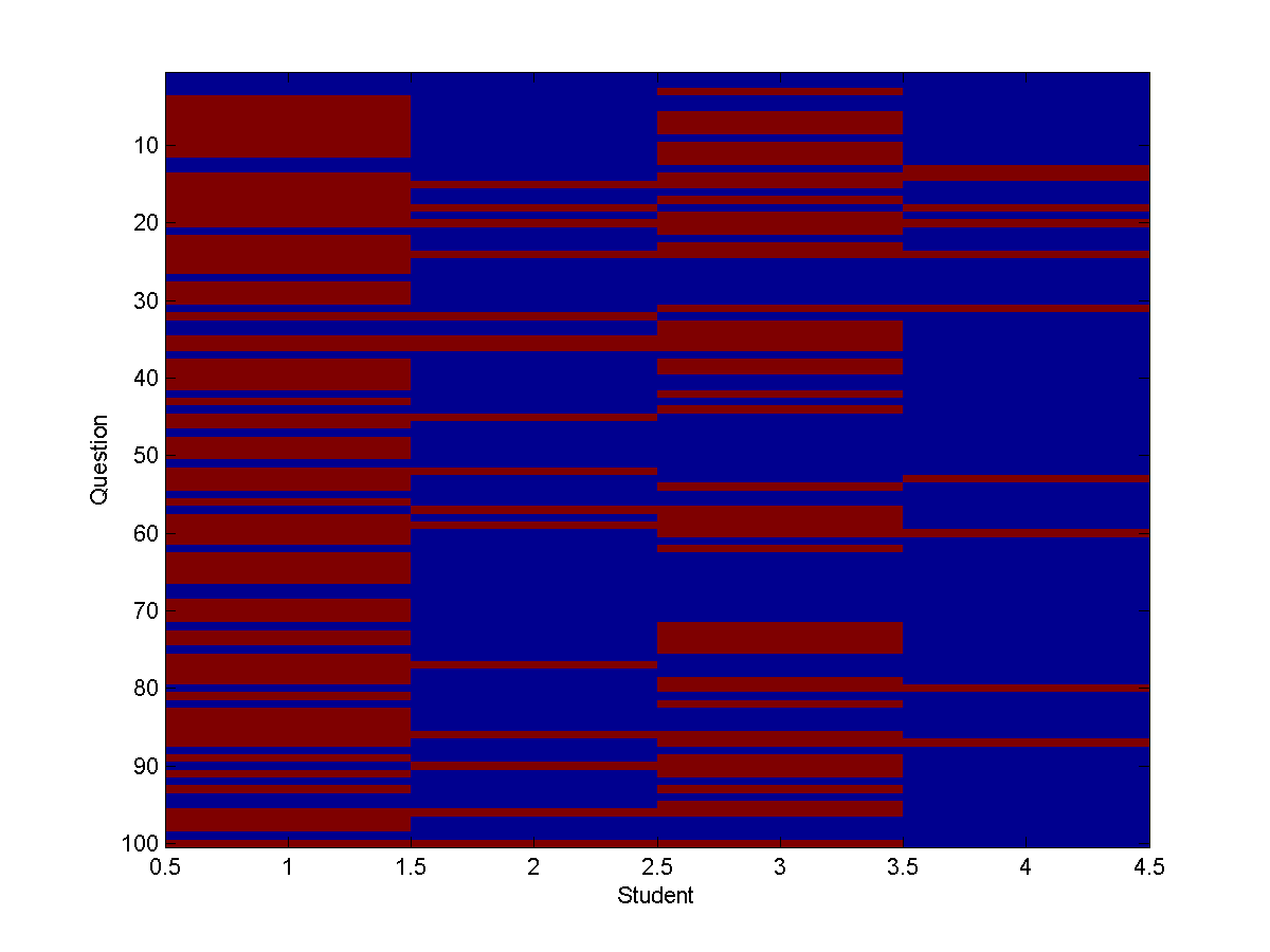
There is clearly a lot more blue in Mark's column in test 2.
Note that generating samples in this way will not in general be the same as sampling all the nodes independently from their marginal distributions. For example, in the above plot we see that in every sample where Heather got the question wrong, either Mark or Allison also got the question wrong.
??? Undefined function or method 'UGM_Decode_ExactC' for input arguments of type 'int32'.
This happens because Matlab could not find the mex file for your operating system (in UGM, files ending with a capital 'C' are mex files). Mex files are compiled C functions that can be called from Matlab. These are useful when the extra speed provided by C (compared to Matlab) is needed. I have written mex versions of some of the parts of UGM that I've used in research projects. Unfortunately, mex files need to be compiled for the operating system that they are being used on. Although UGM includes compiled files for some operating systems, it does not include mex files for all operating systems. If the mex files for your operating system are not included and you get this error, there are two possible solutions:
edgeStruct.useMex = 0;
optimalDecoding = UGM_Decode_Exact(nodePot,edgePot,edgeStruct)
In place of a mex file, it will use the Matlab code that the mex file was based on. All of the mex files in UGM have corresponding Matlab code, since I wanted to maintain easily readable (but equivalent) versions of the files. Setting edgeStruct.useMex to 0 can also be useful for debugging problems, since you will get Matlab errors instead of segmentation violations. However, keeping this field set to 0 should be avoided if possible, since for larger problems the Matlab code might be much slower.