Block UGM Demo
A key aspect of the approximate decoding/inference/sampling methods that we have discussed up to this point is that they are based on performing local calculations. In most cases, this involved updating the state of a single node, conditioning on the values of its neighbors in the graph.
As we discussed in the conditioning and cutset demos, we can do conditional calculations in a UGM by forming a new UGM with some of the edges removed. The previous approximate decoding/inference/sampling take this to the extreme and condition on all nodes except one, so that the conditional UGM consists of a single node (leading to trivial calculations).
However, we might also consider approximate decoding/inference/sampling methods where the conditional UGM is more complicated, but still simple enough that we can do exact calculations.
We will refer to methods that use this simple but powerful idea as block approximate decoding/inference/sampling methods.
Tree-Structured Blocks
The approximate inference methods from the previous demo correspond to the special case where each variable forms its own block. By conditioning on all variables outside the block, it is straightforward to do exact calculations within the block. We want to consider more general blocking schemes, and in particular we will focus on the case of tree-structured blocks.
Rather than having 1024 single-node blocks, it is possible to use just two tree-structured blocks for the noisy X problem. There are many ways to do this, and the diagram below illustrates one of them (the red points on the lattice are one block, the blue points are another):
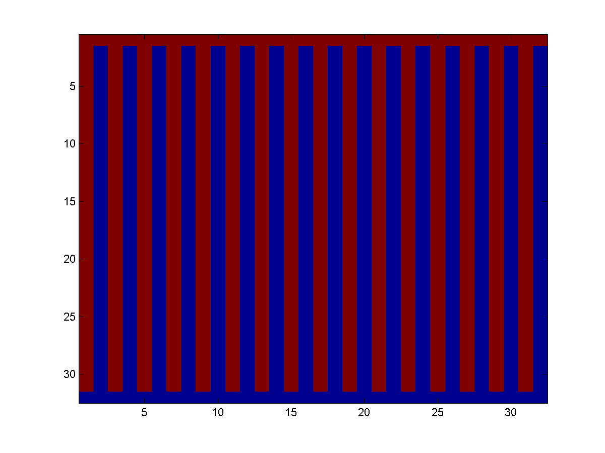
The red blocks form a tree-structured UGM conditioned on the blue blocks, and vice versa. In this case, the blocks form a partition of the nodes, meaning that each variable is in one and only one block. For the block mean field algorithm below, it is important that the blocks form a partition. For the block ICM and Gibbs sampling algorithm, each variable should still be assigned to at least one block, but we can include each variable in more than one block.
In UGM, the blocks are stored in a cell array. We can make the blocks above for the noisy X problem as follows:
getNoisyX
nodeNums = reshape(1:nNodes,nRows,nCols);
blocks1 = zeros(nNodes/2,1);
blocks2 = zeros(nNodes/2,1);
b1Ind = 0;
b2Ind = 0;
for j = 1:nCols
    if mod(j,2) == 1
        blocks1(b1Ind+1:b1Ind+nCols-1) = nodeNums(1:nCols-1,j);
        b1Ind = b1Ind+nCols-1;

        blocks2(b2Ind+1) = nodeNums(nRows,j);
        b2Ind = b2Ind+1;
    else
        blocks1(b1Ind+1) = nodeNums(1,j);
        b1Ind = b1Ind+1;

        blocks2(b2Ind+1:b2Ind+nCols-1) = nodeNums(2:nCols,j);
        b2Ind = b2Ind+nCols-1;
    end
end
blocks = {blocks1;blocks2};
Block ICM
In the ICM approximate decoding algorithm, we cycled through the nodes, computing the optimal value of each node given the values of all the other nodes. The block ICM approximate decoding algorithm is similar, except we cycle through the blocks, computing the optimal value of each block given the values of all variables that are not in the block. If the blocks form trees, then we can compute the optimal block update using the (non-loopy) max-product belief propagation algorithm.
In UGM, the block ICM algorithm takes an anonymous function that will do the conditional decoding of the blocks, and we can use the block ICM algorithm with UGM_Decode_Tree to do the decoding as follows:
BlockICMDecoding = UGM_Decode_Block_ICM(nodePot,edgePot,edgeStruct,blocks,@UGM_Decode_Tree);
Below is an example of the results obtained with ICM compared to block ICM on a sample of the noisy X problem:
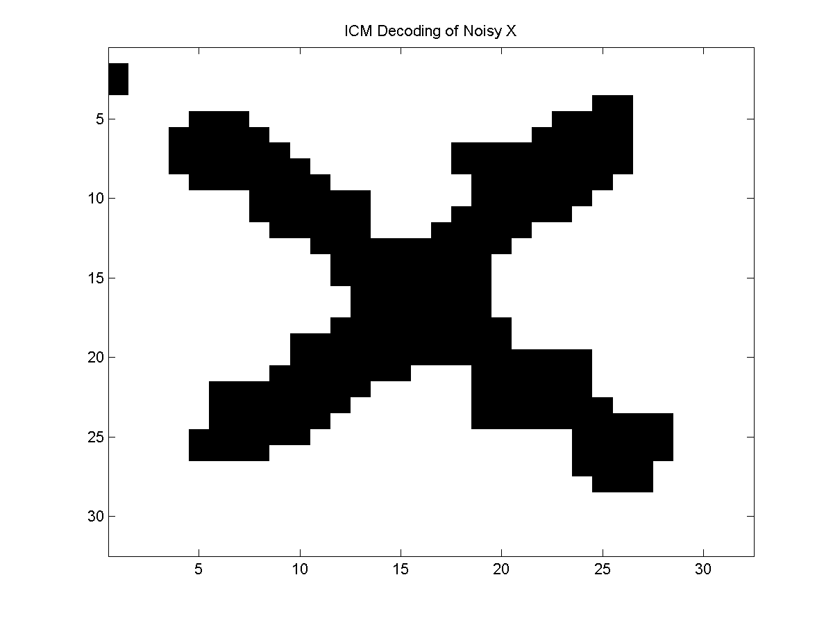
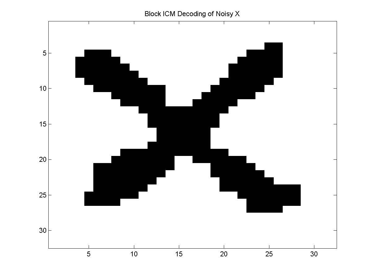
Even though both algorithms used the same initialization and perform simple greedy moves, the more global updates performed in the block method typically lead to better results.
We can even make a comment about the relative 'strengths' of the local optima found by the ICM and block ICM methods. In particular, ICM finds a local optimum in a very weak sense; the approximate decoding found by ICM can not be improved by changing any single state. In contrast, the block ICM algorithm finds a local optimum in a stronger sense; the approximate decoding by block ICM can not be improved by changing any combination of states within any block. Of course, this is still weaker than the decoding given by graph cuts; the graph cuts decoding can not be improved by changing any combination of states (making it the global optimum). But, we can apply block ICM in cases where graph cuts can not be applied. Further, we can improve the strength of the local optimum found by increasing the number of blocks that we consider.
Block Mean Field
The idea of using blocks can also be applied for approximate inference, and we will focus on the case of a block mean field method. In the mean field method, we keep an estimate of the node marginals, and update the marginals for each node by 'mean field conditioning' on all other nodes. In the block mean field method, we keep an estimate of the node marginals, and update the marginals for each block by 'mean field conditioning' on all the nodes outside the block while doing exact inference within the block on the conditional UGM. Here, I'm using the 'scary quotes' around the word conditional because it isn't really conditioning, but is serving a similar purpose. The hope behind this method is that we will get better marginals because we do not need to use a mean field approximation within the blocks.
We can apply the block mean field method using UGM_Infer_Tree for the inference within the blocks using:
[nodeBelBMF,edgeBelBMF,logZBMF] = UGM_Infer_Block_MF(nodePot,edgePot,edgeStruct,blocks,@UGM_Infer_Tree);
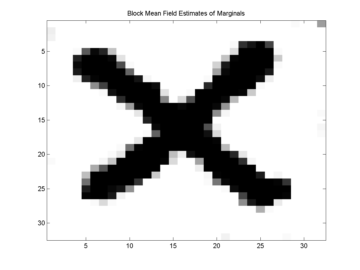
Below, we show the difference between the estimated marginals with the mean field and block mean field method:

In principle we can apply the block mean field method even if the blocks don't form a partition of the nodes. However, this seems like it might further complicate the convergence of the method, since if the blocks don't form a partition then it isn't clear what objective function the updates would be optimizing.
Block Gibbs Sampling
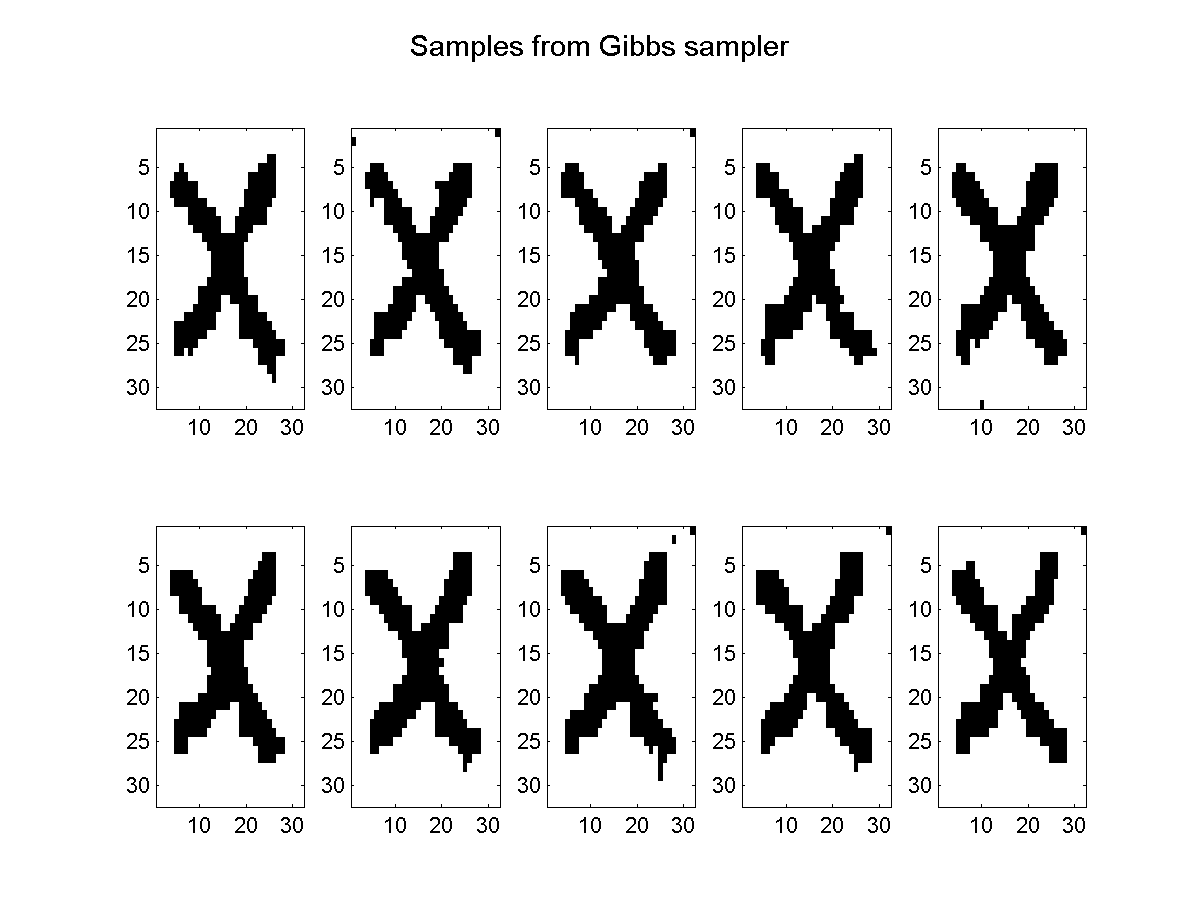
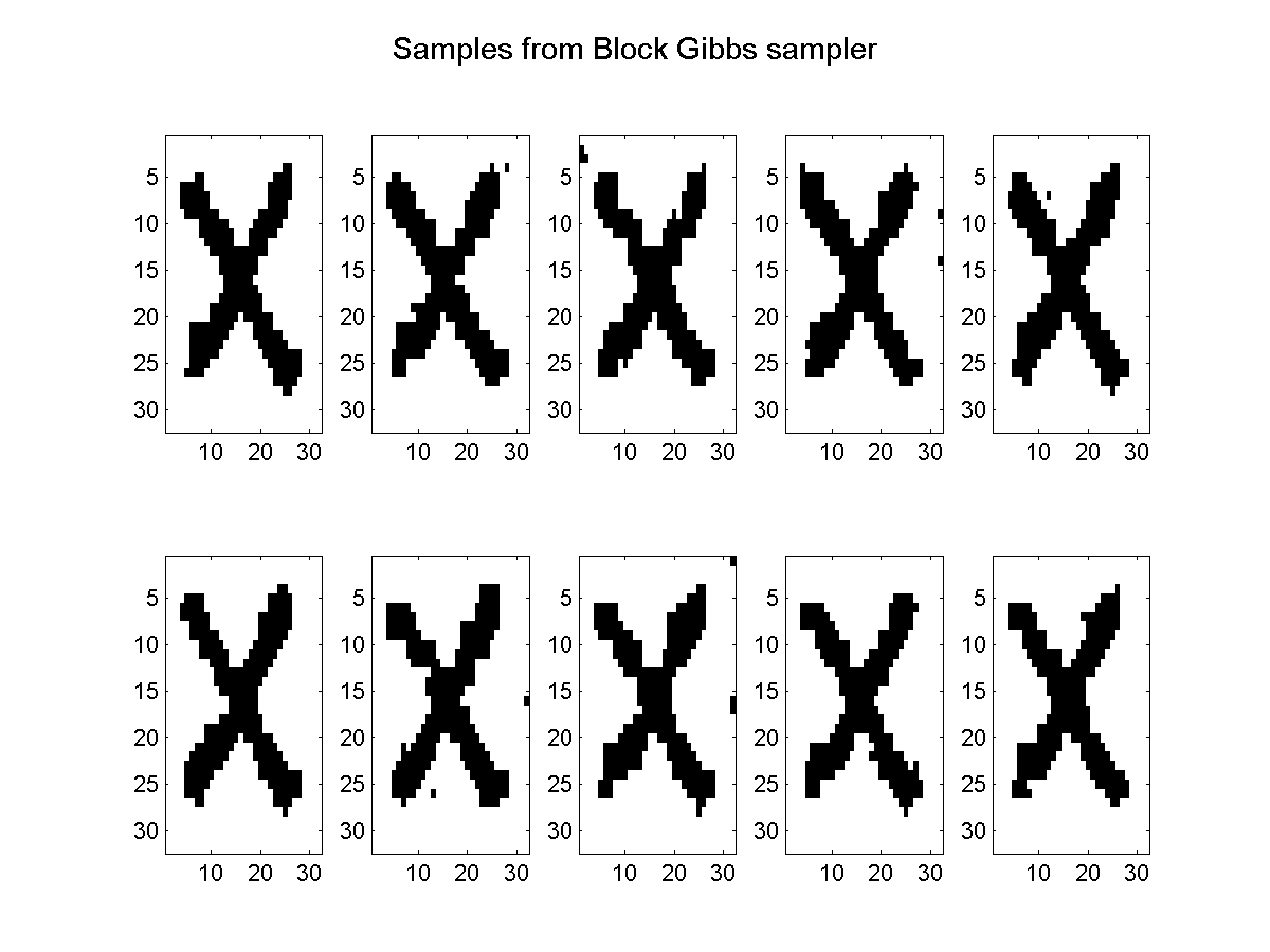
The idea of using blocks can also be used for sampling, and due to their improved performance over the simple Gibbs sampling method, block Gibbs sampling methods are very popular in Bayesian statistics. In this case, the basic idea is again simple but powerful; rather than conditioning on all other variables and sampling a single variable, we condition on all variables outside the block and sample the entire block. To use UGM_Sample_Tree as the sampler within a block Gibbs sampling scheme where we have a burn in of 10 samples and record 20 samples, we can use:
burnIn = 10;
edgeStruct.maxIter = 20;
samplesBlockGibbs = UGM_Sample_Block_Gibbs(nodePot,edgePot,edgeStruct,burnIn,blocks,@UGM_Sample_Tree);
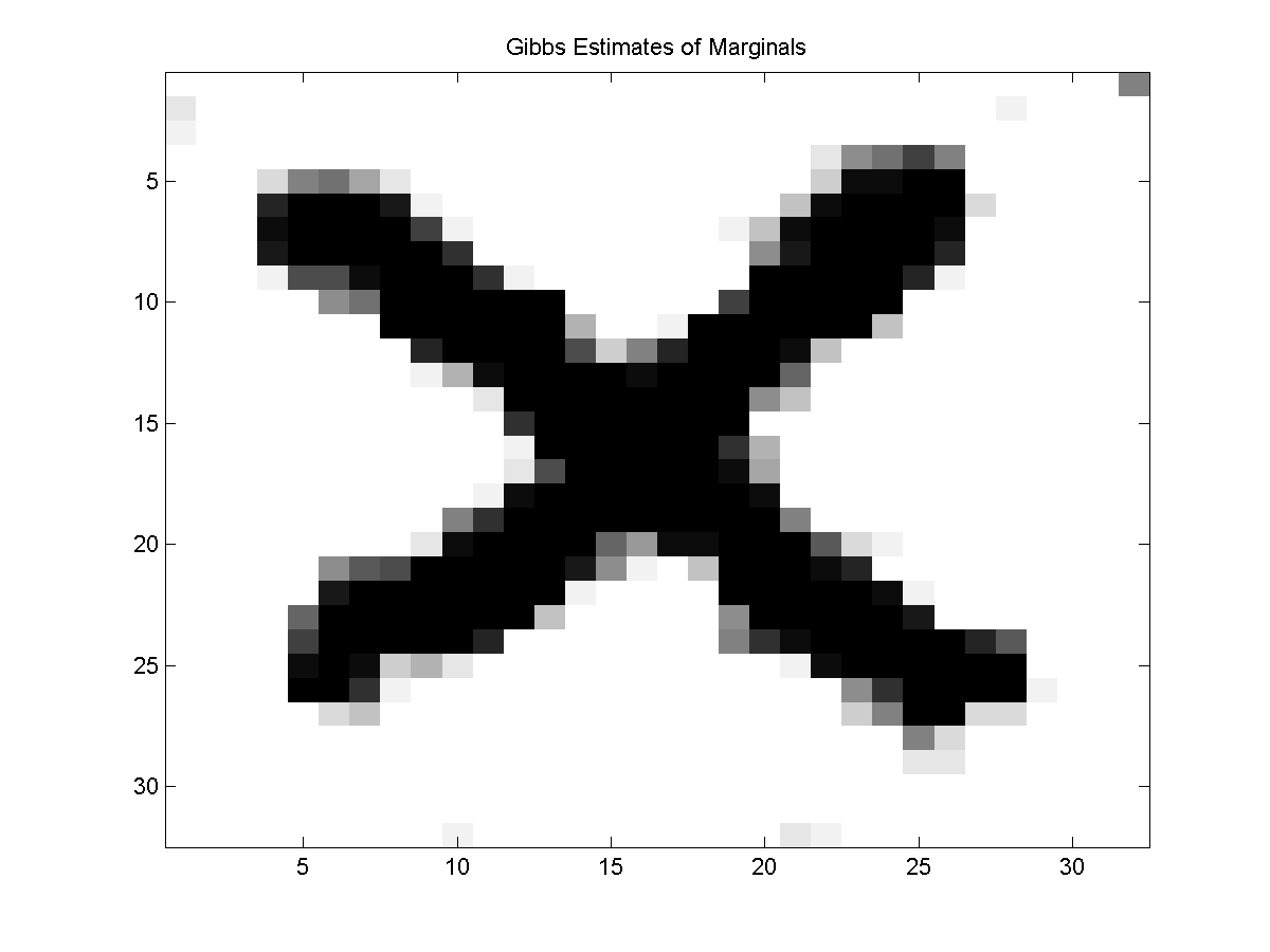
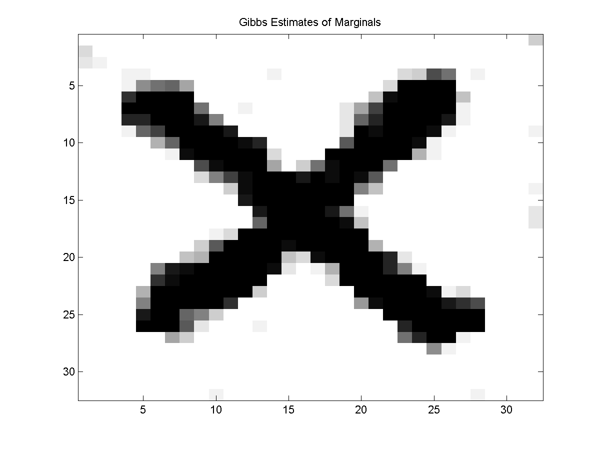
Below we plot every 2nd samples and the estimates of marginals from 20 samples for both the Gibbs sampling method and the block Gibbs sampling method:
Notes
Block versions of mean field methods are attributed to:
- Saul Jordan (1995). Boltmann chains and hidden Markov models. Advances in Neural Information Processing Systems.
Block Gibbs sampling is often attributed to:
- Tannger Wong (1987). The Calculation of Posterior Distributions by Data Augmentation. Journal of the American Statistical Association.
Dividing a 2D lattice into trees and applying block Gibbs sampling is discussed in:
- Hamze de Freitas (2004). From Fields to Trees. Uncertainty in Artificial Intelligence.
As with some other parts of UGM, my implementations of the block methods are fairly slow. This is because my implementation of the tree decoding/sampling/inference isn't particularly optimized, and because the conditional UGM is explicitly constructed to do each block update. In principle, these methods could be implemented to run almost as fast as the regular variants of the methods.
PREVIOUS DEMO NEXT DEMO
Mark Schmidt > Software > UGM > Block Demo