MCMC UGM Demo
The previous demo looked at the ICM algorithm, that iteratively uses decoding of conditionals to give an approximate decoding in the joint model. In this demo we consider the Gibbs sampling algorithm, an analogous method for generating approximate samples.
Markov chain Monte Carlo
Up to this point we have considered sampling algorithms that generate independent samples. That is, the order of the samples did not matter.
MCMC algorithms are different, they generate a set of dependent samples. Specifically, in an MCMC algorithm we use forward sampling of a Markov chain whose stationary distribution is the high-dimensional target distribution we want to sample from. If the Markov chain eventually converges to this stationary distribution, the MCMC samples will start looking like they are distributed according to the target distribution. Theoretically, this happens under very general conditions. Practically, MCMC methods can be thought of as approximate sampling methods for the following reasons:
- If we have a low quality starting state, it may take a long time to reach the stationary distribution. So unless we have a clever initialization (such as the optimal decoding), we may have to throw away a whole bunch of samples before we 'forget' our bad initialization. The initial stage where we throw away samples is sometimes called the burn-in.
- Even if we get to the stationary distribution, we might have to spend a really long time exploring the space before our samples start to look like they are coming from the target distribution.
Gibbs Sampling
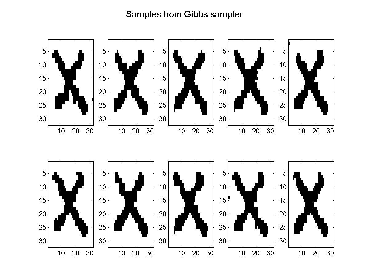
An MCMC sampling scheme that is exhorbitantly popular in statistics is Gibbs sampling. In this algorithm, we start from some intial configuration and we cycle through each node, sampling the state of the node conditioning on all other nodes. After some initial burn-in period where we throw away the samples, we start recording a sample after each pass through the nodes. To run the simple Gibbs sampling algorithm on the noisy X problem to generate 1000 dependent samples after a burn-in of 1000 cycles through the data, we use the following:
getNoisyX;
burnIn = 1000;
edgeStruct.maxIter = 1000;
samplesGibbs = UGM_Sample_Gibbs(nodePot,edgePot,edgeStruct,burnIn);
This function can also take an optional fifth argument that specifies the initial configuration (for example, we might start at the optimal decoding given by the graph cut method, and then set burnIn to zero).
Below, we plot the approximate sample generated after each 100 iterations:
Approximate Sampling for Approximate Decoding/Inference
An approximate sampling method can also be used for approximate decoding. To do this, we simply take the most likely configuration across the samples. The function UGM_Decode_Sample takes an anonymous sampling function, and then gives an approximate decoding by finding the most likely configuration generated by the sampler. To use this function with the Gibbs sampler, we use:
gibbsDecoding = UGM_Decode_Sample(nodePot, edgePot, edgeStruct,@UGM_Sample_Gibbs,burnIn);
In addition to the anonymous sampling function, UGM_Decode_Sample allows a variable length list of additional arguments that are passed in as arguments to the sampling function. In this case, we want it to pass the burnIn variable to the sampling function (we could also give an extra argument giving the initial configuration of the Gibbs sampler).
An example of the approximate decoding produced by this method is:
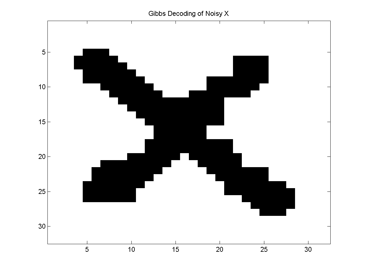
Even though the Gibbs sampler is not trying to find the optimal decoding, it should spend most of its time in high-quality states and this decoding looks fairly good. If used this as an initialization for the ICM decoding algorithm, it might further improve the results.
We can also use sampling methods for inference. For example, we can compute the marginals of the training samples as an approximation to the marginals of the model. We can also compute the sum of the (unique) configurations in the samples as a lower bound on the partition function. The function UGM_Infer_Sample performs these operations using an anonymous sample function:
[gibbsNodeBel,gibbsEdgeBel,gibbsLogZ] = UGM_Infer_Sample(nodePot, edgePot, edgeStruct,@UGM_Sample_Gibbs,burnIn);
Below, we plot the approximate marginals based on the approximate samples:
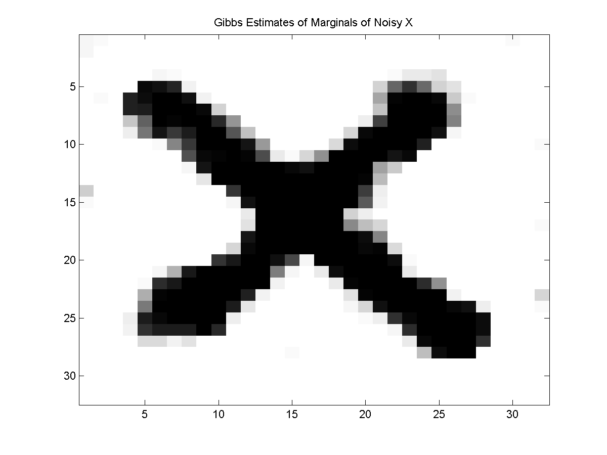
Given that we can 'see' the X in the marginals, we might consider taking the state that maximizes the marginal at each location. Indeed, if we compute the maximum state for each marginal and plot it, we get the following:
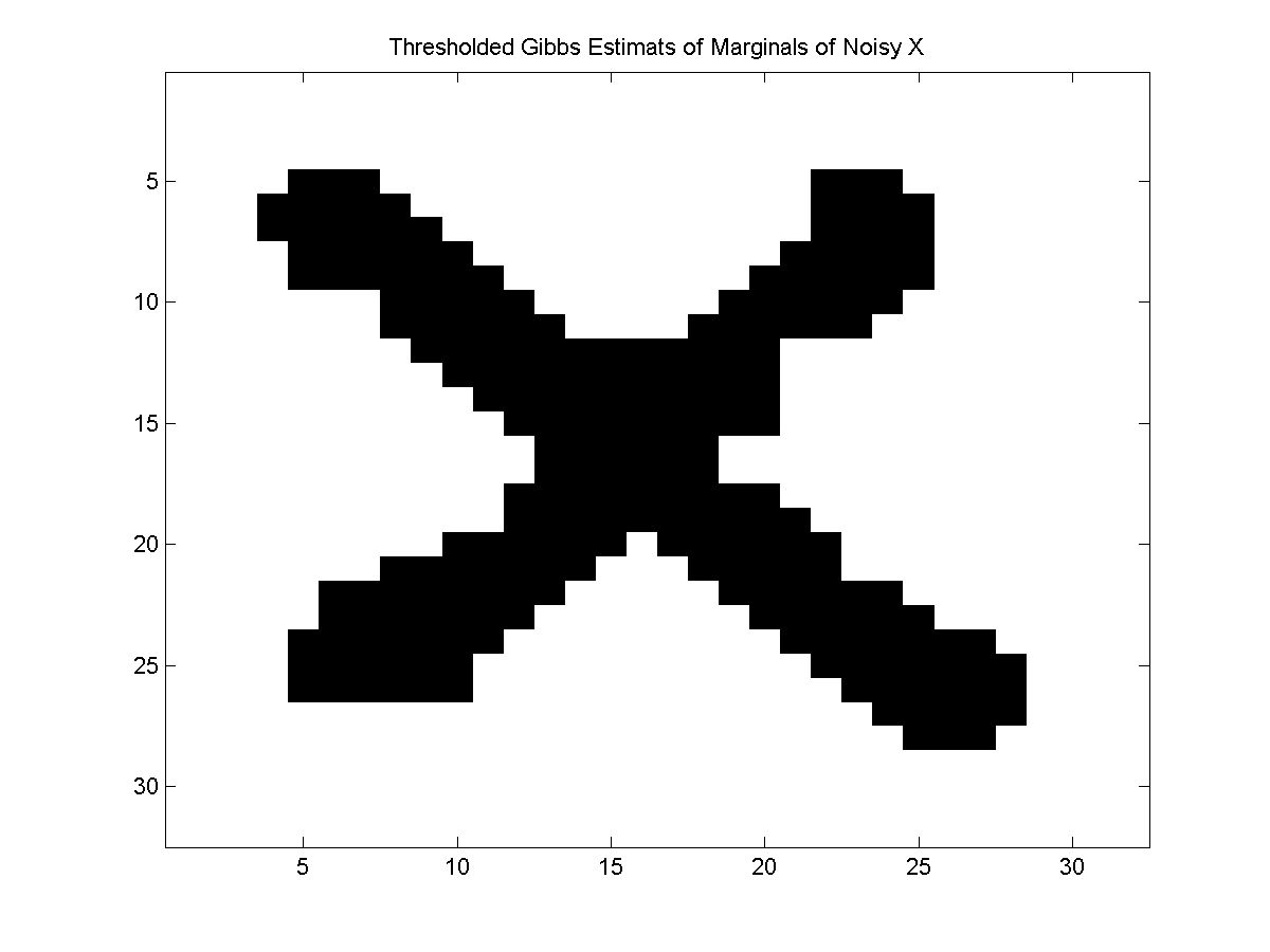
For many models, this type of max of marginals decoding produces more satisfactory results than even the optimal decoding gives. The UGM_Decode_MaxOfMarginals takes an anonymous inference function and implements this particular decoding strategy. This function also takes a variable length argument that specifies the arguments to the inference function. To use the max of marginals decoding where UGM_Infer_Sample is used as the inference function and UGM_Sample_Gibbs is used as UGM_Infer_Sample's sampling function we can use:
maxOfMarginalsGibbsDecode = UGM_Decode_MaxOfMarginals(nodePot,edgePot,edgeStruct,@UGM_Infer_Sample,@UGM_Sample_Gibbs,burnIn);
An alternative strategy to use sampling to generate an approximate decoding is with simulated annealing. In this randomized local search method, we initially allow samples from the conditional to decrease the potential of the current configuration, but over time we eventually require that the potential must increase. Theoretically, if simulated annealing is run for long enough it will yield the optimal decoding. To use an implementation of simulated annealing for approximate decoding we can use:
saDecoding = UGM_Decode_SimAnneal(nodePot, edgePot, edgeStruct);
Notes
Gibbs sampling is one of the very simplest MCMC methods, and it is a special case of the much more general Metropolis-Hastings algorithm. By using different proposal distributions within the Metropolis-Hastings algorithm, it is possible to derive more advanced MCMC methods. For example, in the next demo (on variational methods) we consider a sampler where we augment the simple Gibbs sampler with independent samples from a variational distribution that approximates the original distribution. In the subsequent demo on blocking methods, we consider replacing the simple single-node Gibbs sampling updates with updates that simultaneously sample the states of multiple nodes. These types of extensions can lead to substantial improvements in the quality of the samples.
PREVIOUS DEMO NEXT DEMO
Mark Schmidt > Software > UGM > MCMC Demo