This subsection provides experimental data to compare the VE -based approaches namely PD, TT, and VE1 . We also compare those approaches with VE itself to determine how much can be gained by exploiting causal independencies.
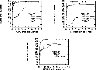
Figure 5: Comparisons in the 364-node BN.
In the 364-node network, three types of queries with one query variable and five, ten, or fifteen observations respectively were considered. Fifty queries were randomly generated for each query type. A query is passed to the algorithms after nodes that are irrelevant to it have been pruned. In general, more observations mean less irrelevant nodes and hence greater difficulty to answer the query. The CPU times the algorithms spent in answering those queries were recorded.
In order to get statistics for all algorithms, CPU time consumption was limited to ten seconds and memory consumption was limited to ten megabytes.
The statistics are shown in Figure 5. In the charts, the curve ``5ve1", for instance, displays the time statistics for VE1 on queries with five observations. Points on the X-axis represent CPU times in seconds. For any time point, the corresponding point on the Y-axis represents the number of five-observation queries that were each answered within the time by VE1 .
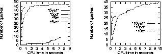
Figure 6: Comparisons in the 422-node BN.
We see that while VE1 was able to answer all the queries, PD and TT were not able to answer some of the ten-observation and fifteen-observation queries. VE was not able to answer a majority of the queries.
To get a feeling about the average performances of the algorithms, regard the curves as representing functions of y, instead of x. The integration, along the Y-axis, of the curve ``10PD", for instance, is roughly the total amount of time PD took to answer all the ten-observation queries that PD was able to answer. Dividing this by the total number of queries answered, one gets the average time PD took to answer a ten-observation query.
It is clear that on average, VE1 performed significantly better than PD and TT, which in turn performed much better than VE . The average performance of PD on five- or ten-observation queries are roughly the same as that of TT, and slightly better on fifteen-observation queries.
In the 422-node network, two types of queries with five or ten observations were considered and fifty queries were generated for each type. The same space and time limits were imposed as in the 364-node networks. Moreover, approximations had to be made; real numbers smaller than 0.00001 were regarded as zero. Since the approximations are the same for all algorithms, the comparisons are fair.
The statistics are shown in Figure 6. The curves ``5ve1" and ``10ve1" are hardly visible because they are very close to the Y-axis.
Again we see that on average, VE1 performed significantly better than PD, PD performed significantly better than TT, and TT performed much better than VE .
One might notice that TT was able to answer thirty nine ten-observation queries, more than that VE1 and PD were able to. This is due to the limit on memory consumption. As we will see in the next subsection, with the memory consumption limit increased to twenty megabytes, VE1 was able to answer forty five ten-observation queries exactly under ten seconds.