This toolbox supports value and policy iteration for discrete MDPs, and includes some grid-world examples from the textbooks by Sutton and Barto, and Russell and Norvig. It does not implement reinforcement learning or POMDPs. For a very similar package, see INRA's matlab MDP toolbox.
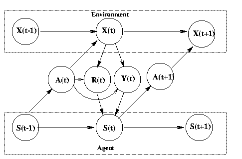
We can formalise the RL problem as follows. The environment is a modelled as a stochastic finite state machine with inputs (actions sent from the agent) and outputs (observations and rewards sent to the agent)
E [ R_0 + g R_1 + g^2 R_2 + ...] = E sum_{t=0}^infty gamma^t R_t
where 0 <= gamma <= 1 is a discount factor which models the
fact future reward is worth less than immediate reward (because
tomorrow you might die). (Mathematically, we need gamma < 1 to make
the infinite sum converge, unless the environment has
absorbing states with zero reward.)

In the special case that Y(t)=X(t), we say the world is fully observable, and the model becomes a Markov Decision Process (MDP). In this case, the agent does not need any internal state (memory) to act optimally. In the more realistic case, where the agent only gets to see part of the world state, the model is called a Partially Observable MDP (POMDP), pronounced "pom-dp". We give a brief introduction to these topics below.
More precisely, let us define the transition matrix and reward functions as follows.
 T(s,a,s') = Pr[S(t+1)=s' | S(t)=s, A(t)=a]
 R(s,a,s') = E[R(t+1)| S(t)=a, A(t)=a, S(t+1)=s']
(We are assuming states, actions and time are discrete. Continuous MDPs can also be defined, but are usually solved by discretization.)
We define the value of performing action a in state s as follows:
Q(s,a) = sum_s' T(s,a,s') [ R(s,a,s') + g V(s') ]where 0 < g <= 1 is the amount by which we discount future rewards, and V(s) is overall value of state s, given by Bellman's equation:
V(s) = max_a Q(s,a) = max_a sum_s' T(s,a,s') [ R(s,a,s') + g V(s) ]In words, the value of a state is the maximum expected reward we will get in that state, plus the expected discounted value of all possible successor states, s'. If we define
R(s,a) = E[ R(s,a,s') ] = sum_{s'} T(s,a,s') R(s,a,s')
the above equation simplifies to the more common form
V(s) = max_a R(s,a) + sum_s' T(s,a,s') g V(s')which, for a fixed policy and a tabular (non-parametric) representation of the V/Q/T/R functions, can be rewritten in matrix-vector form as V = R + g T V Solving these n simultaneous equations is called value determination (n is the number of states).
If V/Q satisfies the Bellman equation, then the greedy policy
p(s) = argmax_a Q(s,a)is optimal. If not, we can set p(s) to argmax_a Q(s,a) and re-evaluate V (and hence Q) and repeat. This is called policy iteration, and is guaranteed to converge to the unique optimal policy. (Here is some Matlab software for solving MDPs using policy iteration.) The best theoretical upper bound on the number of iterations needed by policy iteration is exponential in n (Mansour and Singh, UAI 99), but in practice, the number of steps is O(n). By formulating the problem as a linear program, it can be proved that one can find the optimal policy in polynomial time.
For AI applications, the state is usually defined in terms of state variables. If there are k binary variables, there are n = 2^k states. Typically, there are some independencies between these variables, so that the T/R functions (and hopefully the V/Q functions, too!) are structured; this can be represented using a Dynamic Bayesian Network (DBN), which is like a probabilistic version of a STRIPS rule used in classical AI planning. For details, see
Reinforcement Learning (RL) solves both problems: we can approximately solve an MDP by replacing the sum over all states with a Monte Carlo approximation. In other words, we only update the V/Q functions (using temporal difference (TD) methods) for states that are actually visited while acting in the world. If we keep track of the transitions made and the rewards received, we can also estimate the model as we go, and then "simulate" the effects of actions without having to actually perform them.
There are three fundamental problems that RL must tackle: the exploration-exploitation tradeoff, the problem of delayed reward (credit assignment), and the need to generalize. We will discuss each in turn.
We mentioned that in RL, the agent must make trajectories through the state space to gather statistics. The exploration-exploitation tradeoff is the following: should we explore new (and potentially more rewarding) states, or stick with what we know to be good (exploit existing knowledge)? This problem has been extensively studied in the case of k-armed bandits, which are MDPs with a single state and k actions. The goal is to choose the optimal action to perform in that state, which is analogous to deciding which of the k levers to pull in a k-armed bandit (slot machine). There are some theoretical results (e.g., Gittins' indices), but they do not generalise to the multi-state case.
The problem of delayed reward is well-illustrated by games such as chess or backgammon. The player (agent) makes many moves, and only gets rewarded or punished at the end of the game. Which move in that long sequence was responsible for the win or loss? This is called the credit assignment problem. We can solve it by essentially doing stochastic gradient descent on Bellman's equation, backpropagating the reward signal through the trajectory, and averaging over many trials. This is called temporal difference learning.
It is fundamentally impossible to learn the value of a state before a reward signal has been received. In large state spaces, random exploration might take a long time to reach a rewarding state. The only solution is to define higher-level actions, which can reach the goal more quickly. A canonical example is travel: to get from Berkeley to San Francisco, I first plan at a high level (I decide to drive, say), then at a lower level (I walk to my car), then at a still lower level (how to move my feet), etc. Automatically learning action hierarchies (temporal abstraction) is currently a very active research area.
The last problem we will discuss is generalization: given that we can only visit a subset of the (exponential number) of states, how can know the value of all the states? The most common approach is to approximate the Q/V functions using, say, a neural net. A more promising approach (in my opinion) uses the factored structure of the model to allow safe state abstraction (Dietterich, NIPS'99).
RL is a huge and active subject, and you are recommended to read the references below for more information.
For more details on POMDPs, see Tony Cassandra's POMDP page.