Last updated 10 May 2006.

How to use the CRF2D toolbox

Quick start

After unzipping CRF2D.zip, check that everything installed correctly. Just type the following into matlab, and you should see some pretty pictures, which will be explained below. (Your images may not match the ones shown below due to randomness in the training/ testing set.)

cd CRF2D % wherever you put the zip file
addpath(genpath(pwd)) % assumes matlab 7
demoSingle
demoMulti

If you have a Mac, you may have to compile and put the following mex files onto your path: BP_GeneralComplex_C.mexmac, BP_General_C.mexmac MF_GeneralComplex_C.mexmac.

Toolbox design

Before explaining how to use the toolbox, we give a quick overview of its design principles. The toolbox has several parts:

Feature engine

We currently only implement one feature engine, based on Kumar and Herbert's features. It only works for +1/-1 labels. It is called latticeFeatures, which takes as input a 4D array rawFeatures(d,r,c,s), which specifies the value of feature d for row r, column c, case s. From this, we can create node features as follows:

nodeFeatures(:,i,s) = [1, raw(:,r,c,s))] if expandNode=0
nodeFeatures(:,i,s) = [1, quadratic(raw(:,r,c,s))] if expandNode=1

where i corresponds to node (r,c) and quadratic(v) is a quadratic expansion of the vector v. We can also create edge features using

egdeFeatures(:,e,s) = [1, |raw(:,r,c) - raw(:,r',c')| ] if expandEdge = 0
edgeFeatures(:,e,s) = [1, Quadratic(|raw(:,r,c) - raw(:,r',c')|) ] if expandEdge = 1

where e corresponds to the egde connecting (r,c)-(r',c').

The node potentials are given by

nodepot(xi, i) = exp[ xi w'* nodeFeatures(:,i,s) ]

where xi is the state (+1, -1) of node i, which is in row r, column c. Similiarly, the edge potentials for edge e (connecting nodes i, j) have the form

edgepot(xi,xj,e) = exp[ xi xj v' * edgeFeatures(:,e) ]

The gradient is the observed minus the expected features:

gradNode(:,i,s) = label(i,s)* nodeFeatures(:,i,s)
 - sum_x bel(x,i,s) * x * nodeFeatures(:,i,s)

where bel(x,i,s) = P(X(i)=x|s) is the marginal belief for case s. Similarly,

gradEdge(:,e,s) =  label(i,s)*label(j,s)* edgeFeatures(:,e,s)
   - sum_{x,x'} bel2(x,x',e,s) * x * x' * edgeFeatures(:,e,s)

where bel2(x,x',e,s) = P(X(i)=x,X(j)=x'|s) is the pairwise belief and edge e connects i and j.

Inference engine

We have engines for mean field and loopy belief propagation, which approximate the beliefs mentioned above. These work on arbitrary graph structures (with pairwise potentials), although all the demos currently assume a 2D nearest neighbor lattice. Currently all the code assumes the labels are binary (+1/-1). The code is written in C, since it is not possible to vectorize these algorithms when the edge potentials are non-stationary. (In contrast, for MRFs, one can write fast BP code for lattices in matlab.)

You may also be interested in some matlab/C code for inference in undirected MRFs (with pairwise potentials) by Talya Meltzer.

Objective function

We support pseudo likelihood and conditional likelihood (with quadratic regularization).

Optimizer

We have implemented (annealed) stochastic gradient descent and stochastic meta descent (a way to automatically adapt the step size). But you can also use any other optimizer, such as BFGS (called fminunc in the matlab optimization toolbox), conjugate gradient, etc.

Training and testing on a single image

We now discuss the file demos/demoSingle.m.

Initialization

This demo illustrates how to perform inference, but not learning. It loads the binary 'X' image, and makes a version with noise added:

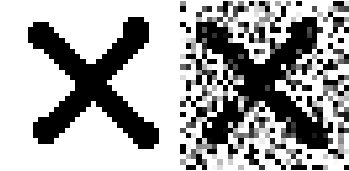
label = sign(double(imread('X.PNG'))-1);
label=label(:,:,1);
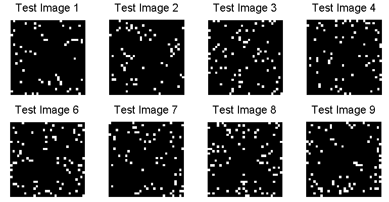
noisy = label+randn(32,32);
imshow([label noisy]);
title('Labels   Observed');

We will use the left image as the class labels (-1 or 1), and the right image as the features at each pixel location. We now want to put this in the appropriate data structure, which we will call 'trainingdata':

featureEng = latticeFeatures(0,0);
features = permute(noisy,[4 1 2 3]);
traindata.nodeFeatures = mkNodeFeatures(featureEng,features);
traindata.edgeFeatures = mkEdgeFeatures(featureEng,features);
traindata.nodeLabels = label;
traindata.ncases = 1;
trainNdx = 1:traindata.ncases;

We first initialize our feature engine object. We have specified (0,0) since we want to use our features directly, as opposed to performing a quadratic basis function expansion. The 'mkNodeFeatures' and 'mkEdgeFeatures' functions put our extracted features in the appropriate format, using the parameters of the feature engine. A location (i,r,c,case) in the 4D array 'features' stores the ith feature for (row r, column c) of image case. The nodeLabels field has the form (r,c,case), and is the class label for (row r, column c) of image case. Here, we have only 1 case. Note that the edge features used in the by this feature engine are the normalized absolute differences between raw edge features at adjacent locations in the lattice.

Before training the model, we select an initial set of parameters (using small random values). Since the objective function is convex, the initial values should not matter very much, but they can affect the numerical stability of approximate inference.

nNodeFeatures = size(traindata.nodeFeatures,1);
nEdgeFeatures = size(traindata.edgeFeatures,1);
weights = initWeights(featureEng,nNodeFeatures,nEdgeFeatures);

Finally, we will try doing inference with our initial parameters (using the mean field approximation for inference):

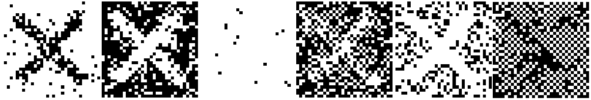
nstates = 2;
infEng = latticeInferMF(nstates);
caseNum = 1;
featureEng = enterEvidence(featureEng, traindata, caseNum); % store data

[nodePot, edgePot] = mkPotentials(featureEng, weights);
[nodeBel, MAPlabels] = infer(infEng, nodePot, edgePot);
imshow(MAPlabels);

Above, we first created a mean field inference engine. We then entered case 1 of our training data into the feature engine. The feature engine subsequently lets us make the node and edge potentials, needed to perform inference with the inference engine. The inference engine returns the node beliefs (marginal probabilities) and assigns labels. Inference with random parameters tends to be a sub-optimal labeling strategy, below are some examples of running this demo:

Pseudo likelihood training

We now discuss how to optimize the pseudo likelihood.

reg = 1;
maxIter = 10;
options = optimset('Display','iter','Diagnostics','off','GradObj','on',...
    'LargeScale','off','MaxFunEval',maxIter);

We specify the pseudolikelihood objective and gradient function, and set up the associated arguments:

gradFunc = @pseudoLikGradient;
gradArgs = {featureEng,traindata,reg};

And we optimize the objective function:

winit = initWeights(featureEng, nNodeFeatures,nEdgeFeatures);
weights = fminunc(gradFunc,winit,options,trainNdx,gradArgs{:});

We can plot the results as before

[nodePot, edgePot] = mkPotentials(featureEng, weights);
[nodeBel, MAPlabels] = infer(infEng, nodePot, edgePot);
imshow(MAPlabels);

For this data set, the optimal pseudolikelihood parameters do not prove to be very interesting (except to show that pseudolikelihood tends to over-smooth, in this case to an all-white image):

Mean field

Now we optimize the conditional likelihood using mean field.

infEng = latticeInferMF(nstates);
gradFunc = @scrfGradient;
gradArgs = {featureEng, infEng, traindata, reg};
weights = fminunc(gradFunc,winit,options,trainNdx,gradArgs{:});

The results are much better.

Belief propagation

We replace the mean field approximation with Loopy Belief Propagation (LBP) for training and inference. This only requires modifying the inference engine used:

infEng = latticeInferBP(nstates);
gradFunc = @scrfGradient;
gradArgs = {featureEng, infEng, traindata, reg};
weights = fminunc(gradFunc,winit,options,trainNdx,gradArgs{:});

Example results of an LBP trained model with LBP inference are shown below:

Median filtering

A classic method (built in to the image processing toolbox) is median filtering.

imshow(medfilt2(noisy)>0)

This gives poor results in this case.

Training and testing on multiple (different) images

We now discuss demos/demoMulti.m. We do not show all the code here; consult the source file for details. This demo illustrates the design of a slightly more interesting experiment. This demo make 50 training images, and 10 test images (all generated from the original X), computes the initial test error, and displays the test images with BP inference using the initial parameters. Below is an example of the initial images:

BFGS+BP

This demo uses BP training on the 50 training images, computes the classification performance using BP inference on the 10 test images, and displays the test image results. In this demo, we run the algorithm for only 3 iterations (each iteration requires performing BP inference 50 times).

reg = 1;
maxIter = 3;
options = optimset('Display','iter','Diagnostics','off','GradObj','on',...
    'LargeScale','off','MaxFunEval',maxIter);

gradFunc = @scrfGradient;
gradArgs = {featureEng, infEng, traindata, reg};

weights = fminunc(gradFunc,winit,options,trainNdx,gradArgs{:});

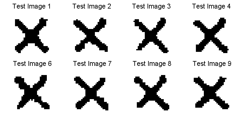
After processing each of the 50 training images 3 times, the batch training procedure does not make significant progress, given the redundency in the data: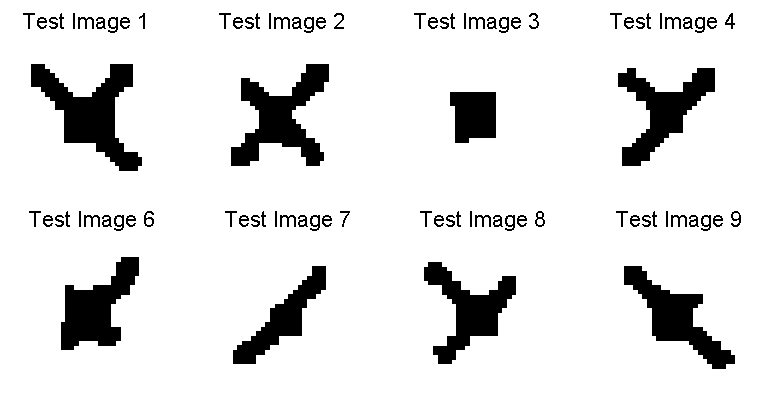

SG+BP

An alternate method of training is to use stochastic gradient methods. After the 3 iteration 3 BFGS training, this demo uses a simple (annealed) stochastic gradient method to update the parameters after looking at each image (or a small subset of the images), starting from the same initial parameters. This demo now requires the specification of a learning rate, mini-batch size, an indicator for whether annealing will be used, and the parameter tau in the expression eta/(t+tau) (if annealing is used, where t is the iteration number):

eta = 0.0001;
batch_size = 1;
anneal = 0;
tau = 0;

Training follows a similar form to the batch scenario:

weights = stochgrad(gradFunc,winit,trainNdx,'gradArgs',gradArgs,...
    'maxIter',maxIter,'eta',eta,'batch_size',batch_size);

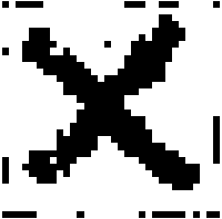
This demo uses only 1 iteration, so training is on-line. Some result images are shown below: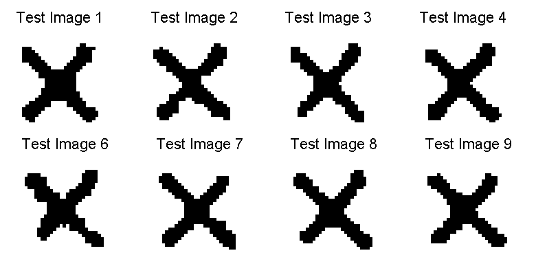

SMD+BP

A disadvantage of the above stochastic method is that it a given learning rate may not converge to the optimal solution, or may do so at too slow of a rate. This demo uses Stochastic Meta-Descent (SMD) to adaptively set the learning rates for the different variables, and takes advantage of the complex plane in the gradient calucation to approximate the Hessian-Vector product in order to incorporate second-order information. This requires two additional parameters, the meta-gain mu and the decay factor lambda:

eta0 = 0.0001;
mu = 0.001;
lambda = 0.9;

Training is done using the following:

weights = smd(gradFunc,winit,trainNdx,'gradArgs',gradArgs,...
    'maxIter',maxIter,'eta0',eta0,'batch_size',batch_size,...
    'lambda', lambda, 'mu', mu);

In this data, we have a very small number of features, so SMD does not give a substantial improvement. Below are some example results for the on-line training scenario after viewing all training images:

Reproducing the DRF experiments

Kumar and Herbert proposed a model called "discriminative random field" (DRF) which is equivalent to a 2D CRF. To details on how to apply the CRF2D toolbox to their data, click here.