"The essence of the Bayesian approach is to provide a mathematical rule explaining how you should change your existing beliefs in the light of new evidence. In other words, it allows scientists to combine new data with their existing knowledge or expertise. The canonical example is to imagine that a precocious newborn observes his first sunset, and wonders whether the sun will rise again or not. He assigns equal prior probabilities to both possible outcomes, and represents this by placing one white and one black marble into a bag. The following day, when the sun rises, the child places another white marble in the bag. The probability that a marble plucked randomly from the bag will be white (ie, the child's degree of belief in future sunrises) has thus gone from a half to two-thirds. After sunrise the next day, the child adds another white marble, and the probability (and thus the degree of belief) goes from two-thirds to three-quarters. And so on. Gradually, the initial belief that the sun is just as likely as not to rise each morning is modified to become a near-certainty that the sun will always rise."
                 likelihood * prior
posterior = ------------------------------
                  marginal likelihood
or, in symbols,
             P(e | R=r) P(R=r)
P(R=r | e) = -----------------
                   P(e)
where P(R=r|e) denotes the probability that random variable R has
value r given evidence e.
The denominator is just a normalizing
constant that ensures the posterior adds up to 1; it can be computed
by summing up the numerator over all possible values of R, i.e.,
P(e) = P(R=0, e) + P(R=1, e) + ... = sum_r P(e | R=r) P(R=r)This is called the marginal likelihood (since we marginalize out over R), and gives the prior probability of the evidence.
Let P(Test=+ve | Disease=true) = 0.95, so the false negative rate, P(Test=-ve | Disease=true), is 5%. Let P(Test=+ve | Disease=false) = 0.05,, so the false positive rate is also 5%. Suppose the disease is rare: P(Disease=true) = 0.01 (1%). Let D denote Disease (R in the above equation) and "T=+ve" denote the positive Test (e in the above equation). Then
                                 P(T=+ve|D=true) * P(D=true)
P(D=true|T=+ve) =  ------------------------------------------------------------
                     P(T=+ve|D=true) * P(D=true)+ P(T=+ve|D=false) * P(D=false)

                   0.95  * 0.01              0.0095
               =  -------------------    =  -------     = 0.161
                  0.95*0.01 + 0.05*0.99      0.0590
So the probability of having the disease given that you tested
positive is just 16%.
This seems too low, but here is an intuitive argument to support it.
Of 100 people, we expect only 1 to have the disease, and that person
will probably test positive.
But we also expect about 5% of the others (about 5 people in total)
to test positive by accident.
So of the 6 people who test positive, we only expect 1 of them to
actually have the disease; and indeed 1/6 is approximately 0.16.
(If you still don't believe this result,
try reading
An Intuitive
Explanation of Bayesian Reasoning
by Eliezer Yudkowsky.)
In other words, the reason the number is so small is that you believed that this is a rare disease; the test has made it 16 times more likely you have the disease (p(D=1|T=1)/p(D=1)=0.16/0.01=16), but it is still unlikely in absolute terms. If you want to be "objective", you can set the prior to uniform (i.e. effectively ignore the prior), and then get
                                 P(T=+ve|D=true) * P(D=true)
P(D=true|T=+ve) =  ------------------------------------------------------------
                                    P(T=+ve)

                   0.95  * 0.5              0.475
               =  -------------------    =  -------     = 0.95
                  0.95*0.5 + 0.05*0.5        0.5
This, of course, is just the true positive rate of the test.
However, this conclusion relies on your belief that, if you did not
conduct the test, half the people in the world have the disease, which
does not seem reasonable.
A better approach is to use a plausible prior (eg P(D=true)=0.01), but then conduct multiple independent tests; if they all show up positive, then the posterior will increase. For example, if we conduct two (conditionally independent) tests T1, T2 with the same reliability, and they are both positive, we get
                                 P(T1=+ve|D=true) * P(T2=+ve|D=true) * P(D=true)
P(D=true|T1=+ve,T2=+ve) =  ------------------------------------------------------------
                                           P(T1=+ve, T2=+ve)

                   0.95  * 0.95 * 0.01                 0.009
               =  -----------------------------    =  -------     = 0.7826
                  0.95*0.95*0.01 + 0.05*0.05*0.99       0.0115
The assumption that the pieces of evidence are conditionally
independent is called the
naive Bayes assumption. This model has been
successfully used for classifying email as spam (D=true) or not
(D=false) given the presence of various key words (Ti=+ve if word i is
in the text, else Ti=-ve).
It is clear that the words are not independent, even conditioned on
spam/not-spam, but the model works surprisingly well nonetheless.
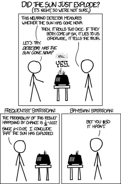
Frequentist statistics suffers from various undesirable counter intuitive properties, due to the fact that it relies on the notion of hypothetical repeated trials, rather than conditioning on the observed evidence. The following cartoon (from xkcd) summarizes the situation quite well:
Bayes Theorem is commonly ascribed to the Reverent Thomas Bayes (1701-1761) who left one hundred pounds in his will to Richard Price ``now I suppose Preacher at Newington Green.'' Price discovered two unpublished essays among Bayes's papers which he forwarded to the Royal Society. This work made little impact, however, until it was independently discovered a few years later by the great French mathematician Laplace. English mathematicians then quickly rediscovered Bayes' work.
Little is known about Bayes and he is considered an enigmatic figure. One leading historian of statistics, Stephen Stigler, has even suggested that Bayes Theorem was really discovered by Nicolas Saunderson, a blind mathematician who was the fourth Lucasian Professor of Mathematics at Cambridge University. (Saunderson was recommended to this chair by Isaac Netwon, the second Lucasian Professor. Recent holders of the chair include the great physicist Paul Dirac and the current holder, Stephen Hawking).